In a recent post, we discussed some basic architectures of CDRs. We’ll now use this short article to discuss a specific architecture, the Baud Rate Mueller-Muller CDR (MMPD). This architecture is widely used in high-speed serial links, and it is known for baud rate operation of low complexity.
Baud Rate CDR
The idea of baud rate CDR is to sample the incoming data at the baud rate, which is the symbol rate of the data. The counterpart of baud rate CDR is oversampling CDR, or edge-sampling CDR which requires samples happening at the edge crossing. For example, the Alexander oversampling BBPD discussed in the previous post is an edge-sampling CDR. It’s worth noting that baud rate CDR means differently than half-rate CDR; the BBPD can acts as a half-rate CDR if the VCO can generate quadrature clocks, but it still samples on the edge.
Mueller-Muller Phase Detector
Kurt H. Mueller and Markus Müller, in their 1976 paper “Timing Recovery in Digital Synchronous Data Receivers”, proposed a timing recovery algorithm that can be used to recover the clock from a data stream. Originally the algorithm was not specifically for CDR, but according to the authors “[The proposed schemes] apply to binary or multilevel PAM signals as well as to partial response signals.”
We analyze a simplified derivation of the algorithm, tailored specifically from a circuit perspective here.
Suppose we have a lossy channel, and we pass an impulse over the channel to the RX. We would like to make sure we sample at the highest point of the impulse response. Assuming the pre-cursor and post-cursor responses are symmetric, then by assuming our pre-cursor sample equals to the post-cursor sample, we are sampling at the optimal point:
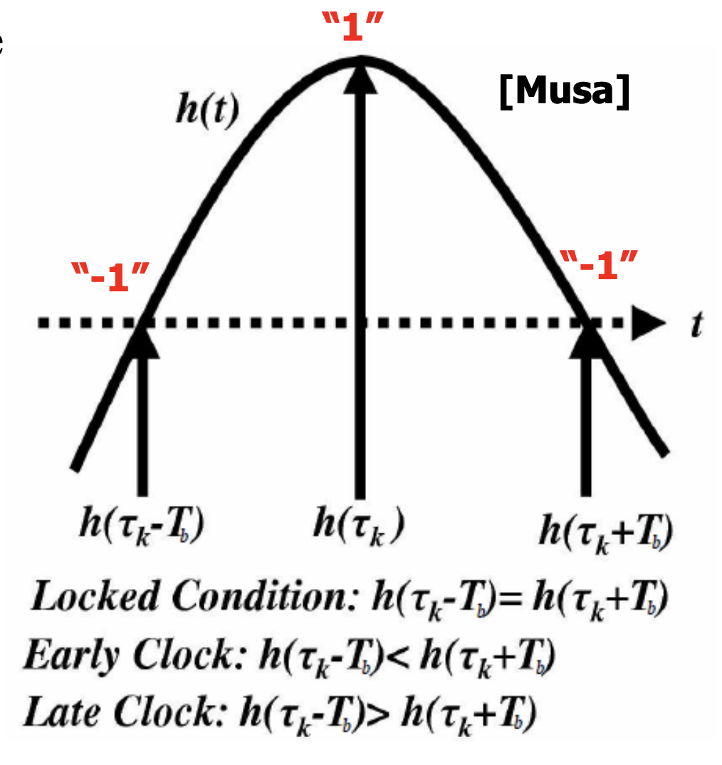
If the channel is lossy, the sampled signal $y_k$ at time index $k$ is the convolution of the channel impulse response $h(t)$ and the transmitted signal $d(t) \in {-1, +1}$, plus some noise $n(t)$:
$$ y_k = \displaystyle \sum_{i=-\infty}^{\infty} h_i d_{k-i} + n_k = \ldots + d_{k+1}h_{-1} + d_k h_0 + d_{k-1}h_1 + \ldots + n_k $$Where:
- $h_0$ is the main cursor
- $h_{-1}$ is the pre-cursor ISI
- $h_1$ is the post-cursor ISI
Now, all CDR protocol will perform data encoding to ensure the DC level of the data stream is half VDD, otherwise the AC coupling will cause the signal to drift. This is also to make sure that there is sufficient data transitions to allow the CDR to recover the clock. For example, 8b/10b encoding is widely used in high-speed serial links. The data stream is encoded such that the number of 1s and 0s are balanced, and the maximum run length of consecutive 1s or 0s is limited. This ensures that there are enough transitions in the data stream for the CDR to lock onto. This leads to the assumption that the transmitted data symbols $d_k$ are independent and identically distributed (i.i.d.) random variables with equal probability of being +1 or -1:
$$ \mathbb{E}[d_i, d_j] = \begin{cases} 1, & i = j \\ 0, & i \neq j \end{cases} $$Additionally, data symbols are uncorrelated with the noise: $\mathbb{E}[d_i n_j] = 0$ for all $i, j$.
Now, if we were to extract the post-cursor ISI $h_1$, we can correlate the sampled $y_k$ with the previous data decision $d_{k-1}$, assuming our BER is sufficiently low:
$$ \mathbb{E}[y_k d_{k-1}] = \mathbb{E}[(\displaystyle \sum_{i=-\infty}^{\infty} h_i d_{k-i} + n_k) d_{k-1}] = \mathbb{E}[h_1 d_{k-1}^2] = h_1 $$Likewise, we can extract the pre-cursor ISI $h_{-1}$ by correlating the sampled $y_k$ with the next data decision $d_{k+1}$:
$$ \mathbb{E}[y_k d_{k+1}] = \mathbb{E}[(\displaystyle \sum_{i=-\infty}^{\infty} h_i d_{k-i} + n_k) d_{k+1}] = \mathbb{E}[h_{-1} d_{k+1}^2] = h_{-1} $$Now given a phase error $\tau$ that’s forcing our sampling instant to drift away from the optimal point, the difference between the pre-cursor and post-cursor ISI will be non-zero. We can use this difference to generate a phase error signal:
$$ f(\tau) = h_1 - h_{-1} = \mathbb{E}[y_k d_{k-1}] - \mathbb{E}[y_k d_{k+1}] $$This function will now provide some physical intuition:
$$ f(\tau) = \begin{cases} 0, & \text{if } \tau = 0 \\ > 0, & \text{if post cursor ISI dominates, or} \ \tau > 0 \\ < 0, & \text{if pre cursor ISI dominates, or} \ \tau < 0 \end{cases} $$Circuit Implementation
Depending on the slope of the transition, $f(\tau)$ will have a different slope when $\tau$ is perturbed around the locking point. Since the slope is sometimes hard to measure, and in actual practice the sampled voltage is hard to digitize (even if we don’t need to digitize the voltage, we still have to do some fast analog processing which is nontrivial), people usually implement the MMPD in a Bang-Bang manner, which is a simple sign detector, i.e. we preserve the sign information of $f(\tau)$, and ignore the magnitude information. This is also known as a binary MMPD.
Shown below is a simple implementation of the binary MMPD:
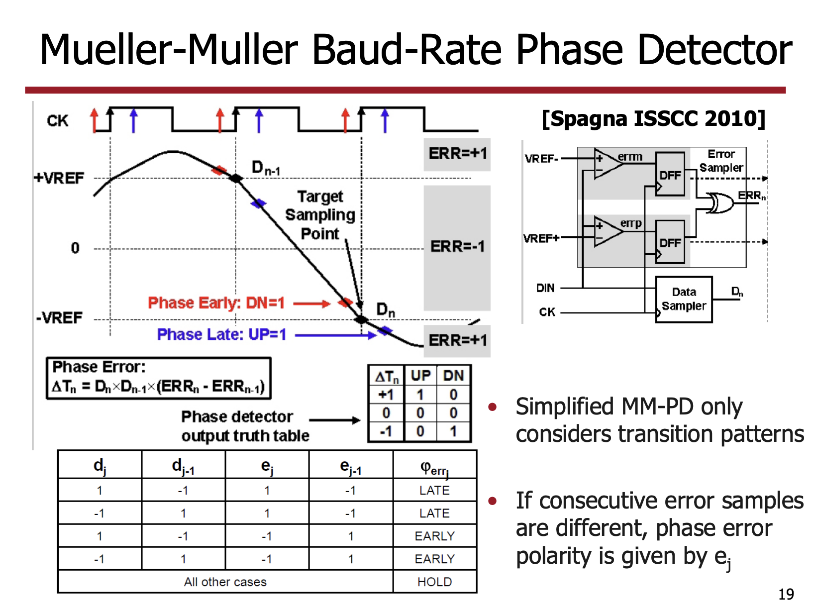
The way to connect the MMPD to our equation is to realize $y_k = h_0 d_k + e_k$, where $e_k$ is the sum of the pre-cursor and post-cursor ISI plus noise. Then we can rewrite the phase error signal as:
$$\mathbb{y_k d_{k-1}} = \mathbb{E}[(h_0 d_k + e_k) d_{k-1}] = \mathbb{E}(e_k d_{k-1})$$Likewise for another term, but we will have to perform one-step delay on the $d_{k+1}$ term to align the timing. The resulting phase error signal is:
$$ \Delta T_n \propto \text{sgn}(e_k d_{k-1}) - \text{sgn}(e_{k-1} d_k) $$Where $\Delta T_n$ is the phase error signal that will be used to adjust the VCO frequency. The sgn function is the sign function, which outputs +1 for positive inputs and -1 for negative inputs.
Gain of the MMPD
The phase detector gain $K_{PD}$ is defined as the slope of the phase error characteristic $f(\tau)$ evaluated at the locking point $\tau = 0$:
$$ K_{PD} = \left. \frac{df(\tau)}{d\tau} \right|_{\tau=0} $$For the linear MMPD, since $f(\tau) = h_1(\tau) - h_{-1}(\tau)$, and the ISI taps are simply the channel pulse response $p(t)$ evaluated at shifted sampling instants — $h_1(\tau) = p(T + \tau)$ and $h_{-1}(\tau) = p(-T + \tau)$ — the gain becomes:
$$ K_{PD} = p'(T) - p'(-T) $$If $p(t)$ is symmetric around $t = 0$ (the ideal sampling instant), then $p’(T) = -p’(-T)$, which simplifies to $K_{PD} = 2p’(T)$. A steeper pulse response roll-off at $t = T$ yields higher PD gain and a more responsive loop.
For the binary (bang-bang) MMPD, the gain is no longer a fixed slope but a linearized quantity that depends on the operating condition. Because the sgn function discards magnitude information, the effective gain is proportional to the probability density of the decision variable crossing zero — essentially, how often the sampler sees a marginally resolved bit near a transition. Concretely:
$$ K_{PD,BB} \approx 2 \cdot p_T \cdot \frac{1}{\sigma_e} \phi\!\left(0\right) $$where $p_T = 0.5$ is the transition probability for i.i.d. data, $\sigma_e$ is the standard deviation of the residual ISI plus noise at the edge sample, and $\phi(0)$ is the PDF of the normalized edge sample evaluated at zero. Unlike the linear MMPD, the BB gain is signal- and noise-dependent, which is the fundamental reason bang-bang CDRs exhibit limit-cycle jitter even at steady state — the loop never truly settles, but instead oscillates within a bounded phase window determined by the loop gain and the intrinsic noise.