Periodogram
We discussed in 相位噪声与抖动的关系 that, we’ll have to convert a time-domain signal into the power spectral density (PSD) to analyze its frequency content. Jitter is in time domain, and phase noise is the scaled version in the frequency domain.
The FFT of an autocorrelation function of a signal is also known as the periodogram:
$$ \mathbb{F}\{x(t)\ast x^*(t)\} = X(f)X^*(f) = |X(f)|^2 $$We know the following theorem from signal processing:
Theorem: The FFT of a real-valued signal is conjugate symmetric (or known as Hermitian symmetry) i.e.,
$$ X(-f) = X^*(f) $$
From there, we can conclude that the periodogram of a real-valued signal must be real-valued and symmetric about zero frequency. This satisfies our expectation that the power spectral density of a real-valued signal should be non-negative and symmetric.
The Periodogram in Discrete Time
In practice we don’t have $x(t)$, only $N$ samples $x[n]$ taken at a sampling rate $f_s$. Taking the FFT:
$$ X[k] = \sum_{n=0}^{N-1} x[n] e^{-j 2\pi k n / N}, \quad f_k = \frac{k f_s}{N} $$the one-sided periodogram is defined as
$$ P[k] = \frac{2}{N f_s} |X[k]|^2, \quad 0 < f_k < \frac{f_s}{2} $$The factor of 2 folds the negative frequencies onto the positive ones, which we can do because of the conjugate symmetry above (DC and Nyquist bins are not doubled). Dividing by $N f_s$ gives us units$^2$/Hz, so that summing $P[k]$ over all bins times the bin width $f_s / N$ gives back the average power of the signal, i.e. Parseval’s theorem.
Example: Periodogram of a Random Walk
Let’s try this on a random walk, or Bronian motion:
$$ x[n] = x[n-1] + w[n], \quad w[n] \sim \mathcal{N}(0, \sigma^2) $$which is just integrated white noise. This is also how the phase of a free-running oscillator behaves in its $1/f^2$ region, so it’s a familiar signal for PLL designers. The integrator has a transfer function of $1/(1 - z^{-1})$, so the white noise PSD $2\sigma^2 / f_s$ is shaped into
$$ S(f) = \frac{2\sigma^2 / f_s}{|1 - e^{-j 2\pi f / f_s}|^2} = \frac{\sigma^2}{2 f_s \sin^2(\pi f / f_s)} \approx \frac{\sigma^2 f_s}{2\pi^2 f^2} \quad (f \ll f_s) $$which rolls off at $-20$ dB/dec, same as the phase noise of an oscillator. Strictly speaking a random walk is not stationary because its variance keeps growing, but $S(f)$ is still the standard way to describe its spectrum, and it’s what our periodogram should converge to.
I generated a random walk with $\sigma = 1$ and $f_s = 1$ kHz, and computed its periodogram:
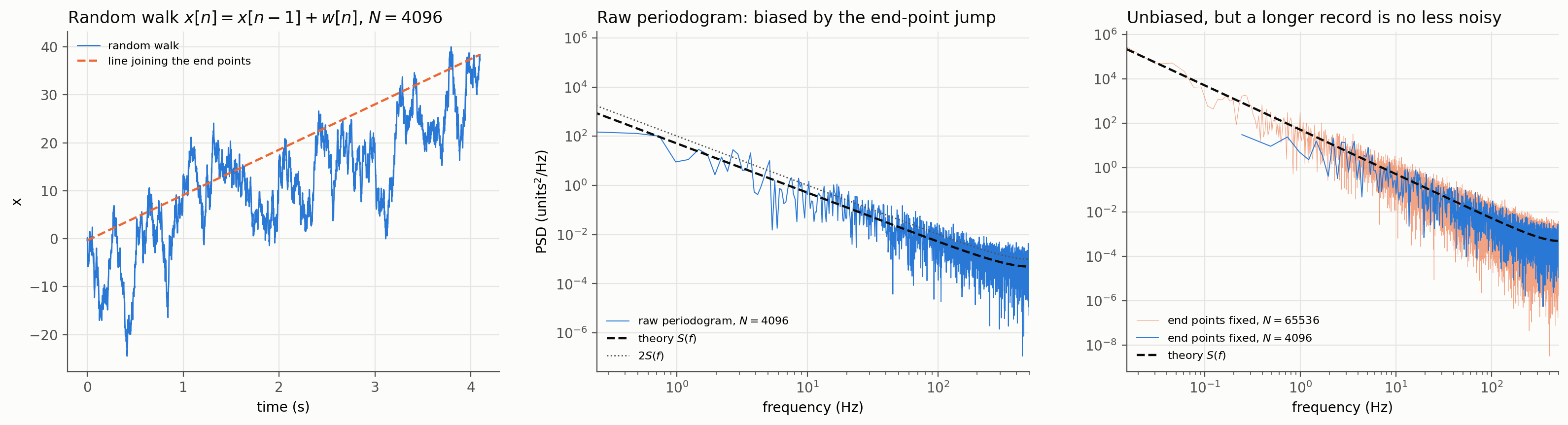
We can see two problems here.
First, the raw periodogram is biased. In the middle plot it sits above the theoretical $S(f)$, and if we average over 400 independent random walks, it comes out at about twice the true value (1.85 times in this run). The reason is shown in the left plot. The FFT assumes the signal is periodic, which means the end of the record is connected back to its beginning. A random walk usually ends up about $\sigma\sqrt{N}$ away from where it started, so this periodic extension has a big jump at the boundary. The jump itself has a $1/f^2$ spectrum with roughly the same magnitude as the random walk, and it adds on top of the true PSD. If we remove the straight line connecting the two end points (the dashed line) before the FFT, the bias goes away, and the average over 400 realizations becomes 1.00 times the theory.
Second, the periodogram is very noisy, and a longer record doesn’t help. Even without the bias, each bin scatters a lot around the theory. The standard deviation of each bin is as large as its mean, because each bin follows an exponential distribution, and 90% of the bins land somewhere between 13 dB below and 5 dB above the true value. In the right plot I used 16 times more data, $N = 65536$ instead of 4096. We get 16 times more bins and therefore finer frequency resolution, but each bin is just as noisy as before: the spread is still $-13$ dB to $+5$ dB. In statistics terms, the periodogram is an inconsistent estimator, meaning its variance doesn’t go to zero as $N \to \infty$.
Both problems are what Welch’s method is designed to fix.
Welch’s Method
Peter Welch proposed this method in 1967 as a way to reduce the variance of the periodogram while maintaining reasonable frequency resolution. The original paper can be found here.
The idea of Welch’s method is simple: since one long periodogram is too noisy, let’s chop the record into shorter segments, compute a periodogram for each segment, and average them.
Suppose we cut the $N$ samples into $K$ segments of length $L$, where neighboring segments start $D$ samples apart (if $D < L$, the segments overlap). Each segment is multiplied by a window $w[n]$ before the FFT:
$$ x_i[n] = w[n] \, x[n + iD], \quad n = 0, \ldots, L-1, \quad i = 0, \ldots, K-1 $$The periodogram of each segment is
$$ P_i[k] = \frac{2}{f_s U} \left| \sum_{n=0}^{L-1} x_i[n] e^{-j 2\pi k n / L} \right|^2, \quad U = \sum_{n=0}^{L-1} w^2[n] $$where $U$ normalizes the power that the window takes away (for a rectangular window $U = L$, which brings us back to the periodogram formula above). Finally, the Welch estimate is just the average:
$$ P_W[k] = \frac{1}{K} \sum_{i=0}^{K-1} P_i[k] $$Averaging $K$ independent periodograms reduces the variance by a factor of $K$. With 50% overlap, neighboring segments are not completely independent, but we get almost twice as many segments out of the same data, which is why 50% overlap with a Hann window is the most common setting.
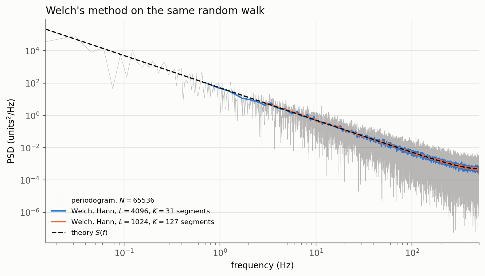
Let’s apply it to the same random walk with $N = 65536$:
| Method | Segments $K$ | Bin spacing | 90% of bins within |
|---|---|---|---|
| Periodogram, $N = 65536$ | 1 | 0.015 Hz | $-12.9$ dB to $+4.8$ dB |
| Welch, Hann, $L = 4096$ | 31 | 0.24 Hz | $-1.5$ dB to $+1.2$ dB |
| Welch, Hann, $L = 1024$ | 127 | 0.98 Hz | $-0.7$ dB to $+0.6$ dB |
Both Welch estimates sit right on the theory, and the scatter drops from almost 18 dB to 2.7 dB and 1.3 dB respectively. Bear in mind that this is not free: we traded frequency resolution for variance. With $L = 1024$ the bins are 1 Hz apart, and the estimate is only usable from a few Hz and above, while $L = 4096$ goes down to below 1 Hz but is noisier. The lowest frequency we can trust is a few bins above DC, i.e. a few times $f_s / L$, because the first couple of bins fall inside the main lobe of the window around DC.
This trade-off is exactly what we face when we measure phase noise from a simulated jitter sequence: a long segment lets us see close-in offsets, and a short segment gives a smooth curve, so the segment length should be picked based on the lowest offset frequency we care about.
Window Selection
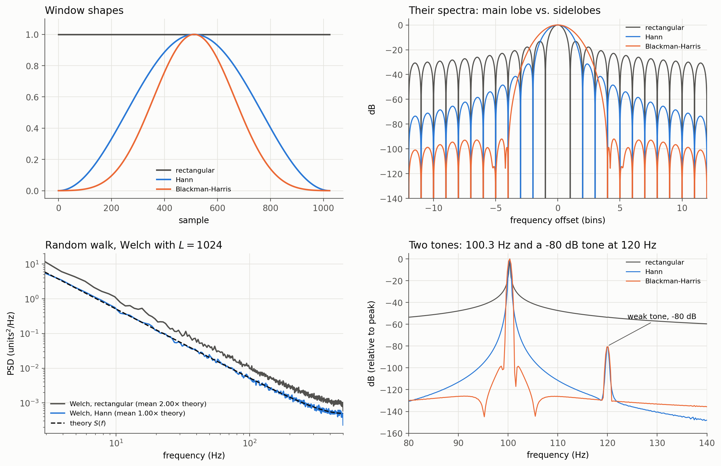
When we cut a segment out of a long signal, we are already applying a rectangular window, whether we like it or not. In the frequency domain, multiplying by a window means convolving the true spectrum with the spectrum of the window, so every window spreads the power of each frequency into its neighbors. This is called spectral leakage. A window spectrum has a main lobe and sidelobes, and different windows trade one against the other:
| Window | Main lobe half-width | Peak sidelobe | Noise bandwidth |
|---|---|---|---|
| Rectangular | 1 bin | $-13$ dB | 1.0 bin |
| Hann | 2 bins | $-31$ dB | 1.5 bins |
| Blackman-Harris | 4 bins | $-92$ dB | 2.0 bins |
A wider main lobe blurs nearby frequencies together, while higher sidelobes let strong components leak far away and hide weak ones. The two examples at the bottom of the figure show why this matters.
Random walk. With a rectangular window, Welch’s method is biased by exactly the same mechanism as before: every segment has its own jump between its end points, and its estimate comes out at 2.00 times the theory. A Hann window tapers each segment to zero at both ends, so the jump disappears, and the estimate is 1.00 times the theory. The rectangular window’s sidelobes only decay at $-20$ dB/dec, which is the same slope as the random walk itself, so the leakage from low frequencies never falls below the true spectrum. For any spectrum that falls at $-20$ dB/dec or steeper, which includes basically all oscillator phase noise, the rectangular window is a bad choice.
Two tones. This is the classic ADC test: a strong tone at 100.3 Hz (not exactly on a bin) and a weak tone 80 dB lower at 120 Hz. With a rectangular window, the leakage skirt of the strong tone is still around $-54$ dB at 120 Hz, and the weak tone is completely buried. With Hann or Blackman-Harris the weak tone shows up clearly, and Blackman-Harris keeps the floor around the strong tone much lower. This is why Blackman-Harris windows are commonly used when measuring the SFDR of an ADC.
WarningThe window also changes the scaling. For a noise PSD, we normalize by $U = \sum w^2[n]$ as in the formula above, so the total noise power is preserved. For the amplitude of a tone, we have to normalize by $(\sum w[n])^2$ instead. Mixing these two up gives errors of a couple of dB (1.8 dB for Hann), which is easy to miss. In
scipy.signal.welch, these arescaling='density'andscaling='spectrum'respectively.
As a rule of thumb: use a Hann window with 50% overlap for noise, use Blackman-Harris when we need a large dynamic range between tones, and only use a rectangular window when the signal contains an exact integer number of periods in each segment (coherent sampling), so that there is no leakage to begin with.