Although I’m an IC designer, it’s sometimes necessary to understand what my EDA tool is doing under the hood, especially when the simulation takes so long for extracted simulation. You might wonder why the extracted simulation takes so much longer than the schematic simulation by just adding a bunch of parasitic elements. The reason lies in the numerical methods used to solve the underlying differential equations, which become more complex and computationally intensive as the circuit model becomes more detailed.
I will discuss some of the commonly used numerical methods used in transient simulation of circuits in this post.
Initial Value Problem (IVP)
Let’s say you want to measure an RC circuit’s settling time after it’s subjected to a step current input, and you ask the simulator to simulate for 50ns. You have just created an initial value problem (IVP), where the initial condition is the circuit’s state at the beginning of the simulation, and the goal is to find the circuit’s state at subsequent time points.
Mathematically, an IVP can be expressed as:
$$ \frac{d\mathbf{x}(t)}{dt} = \mathbf{f}(\mathbf{x}(t), t), \quad \mathbf{x}(t_0) = \mathbf{x}_0 $$where $\mathbf{x}(t)$ represents the state vector of the circuit at time $t$, $\mathbf{f}(\mathbf{x}(t), t)$ represents the system of differential equations governing the circuit, $t_0$ is the initial time, and $\mathbf{x}_0$ is the initial state of the circuit.
The IVP problem can also be interpreted as we performing a mapping from the initial state $\mathbf{x}_0$ at time $t_0$ to the solution vector $\mathbf{x}(t)$ at subsequent time points. In this case, people usually define it in following form:
Given the system
$$ \dot{x} = f(x, t), \quad x(t_0) = x_0 \in \mathbb{R} $$Define mapping $ \psi: \mathbb{R}^n \to \mathbb{C}^n $ such that
$$ \psi(x_0)(t) = x(t, t_0, x_0) \quad \text{for} \quad t \ge t_0 $$
A system must be Lipschitz continuous with respect to the state vector $\mathbf{x}$ to guarantee the existence and uniqueness of the solution to the IVP. This can be either local or global, and whether a solution exists globally or only locally also depends on the Lipschitz condition. This is also known as the Picard-Lindelöf theorem, also known as the uniqueness and existence theorem for ordinary differential equations.
Forward Euler Method
The Forward Euler Method is one of the simplest and most widely used numerical methods for solving IVPs. It is an explicit method, meaning that the state at the next time step is computed directly from the state at the current time step. The method can be expressed as:
$$ x_{k+1} = x_k + h f(x_k, t_k) $$where $x_k$ is the state at time $t_k$, $h$ is the time step size, and $f(x_k, t_k)$ is the derivative of the state with respect to time evaluated at the current state and time.
The Forward Euler Method is conditionally stable, meaning that the choice of time step $h$ can affect the accuracy and stability of the solution. For stiff problems, where the system exhibits rapid changes in some components, the Forward Euler Method may require very small time steps to maintain stability, making it computationally expensive.
Here is a python code snippet demonstrating the Forward Euler Method:
 1import numpy as np
 2
 3def forward_euler(f, x0, t0, t_end, h):
 4    """Solve dx/dt = f(x, t), x(t0) = x0 with x_{k+1} = x_k + h * f(x_k, t_k)."""
 5    n_steps = int(round((t_end - t0) / h))
 6    t = t0 + h * np.arange(n_steps + 1)
 7    x = np.zeros((n_steps + 1,) + np.shape(x0))
 8    x[0] = x0
 9    for k in range(n_steps):
10        x[k + 1] = x[k] + h * f(x[k], t[k])
11    return t, x
12
13# RC circuit driven by a step current: C dv/dt = I - v/R
14R, C, I = 10e3, 1e-12, 100e-6           # 10 kOhm, 1 pF, 100 uA  ->  tau = RC = 10 ns
15tau = R * C
16f = lambda v, t: (I - v / R) / C
17
18t, v = forward_euler(f, x0=0.0, t0=0.0, t_end=50e-9, h=0.1 * tau)
19
20v_exact = I * R * (1 - np.exp(-t / tau))
21print(f"final value: {v[-1]:.4f} V (exact {v_exact[-1]:.4f} V), "
22      f"max error: {np.max(np.abs(v - v_exact)) * 1e3:.2f} mV")
With $h = 0.1\tau$, the final value is 0.9948 V against the exact 0.9933 V, and the worst-case error along the waveform is about 19 mV. Not bad for three lines of math.
Stability: the Test Equation
What does “conditionally stable” actually mean? The standard way to answer this is to feed the method the simplest possible linear system, also known as the test equation:
$$ \dot{x} = \lambda x, \quad \lambda \in \mathbb{C} $$Most linear circuits can be diagonalized into a bunch of these, with $\lambda$ being the poles of the circuit. Applying Forward Euler:
$$ x_{k+1} = x_k + h \lambda x_k = (1 + h\lambda) x_k $$so after $k$ steps we have $x_k = (1 + h\lambda)^k x_0$. Let’s define $z = h\lambda$, and call $R(z) = 1 + z$ the stability function of the method. The numerical solution only decays (like a stable circuit should) if $|R(z)| < 1$, i.e. $z$ has to sit inside a unit circle centered at $-1$.
For our RC circuit, $\lambda = -1/\tau$, therefore:
$$ |1 - h/\tau| < 1 \Rightarrow h < 2\tau $$If we pick a time step larger than $2\tau$, the simulation blows up, even though the circuit itself is perfectly stable. Bear in mind that this limit is set by the fastest pole in the system, not the one we care about.
Backward Euler Method
What if we evaluate the derivative at the end of the step instead of the beginning?
$$ x_{k+1} = x_k + h f(x_{k+1}, t_{k+1}) $$We realize that $x_{k+1}$ now shows up on both sides of the equation, which makes Backward Euler an implicit method: we can’t just compute the next state, we have to solve for it. For a nonlinear $f$, this is done using Newton-Raphson iteration at every time step, which is exactly what your circuit simulator is doing.
Applying the test equation:
$$ x_{k+1} = x_k + h\lambda x_{k+1} \Rightarrow R(z) = \frac{1}{1 - z} $$$|R(z)| < 1$ whenever $\Re(z) < 0$, meaning that Backward Euler is stable for any step size, as long as the circuit itself is stable. This property is called A-stability. On top of that, $R(z) \to 0$ as $z \to -\infty$, so very fast poles are damped out immediately instead of lingering around; this stronger property is called L-stability.
Since the time-marching loop is the same for every method, from now on let’s split it out, and only write down how one step is taken:
 1def integrate(step, f, x0, t0, t_end, h):
 2    """March x_{k+1} = step(f, x_k, t_k, h) from t0 to t_end."""
 3    n_steps = int(round((t_end - t0) / h))
 4    t = t0 + h * np.arange(n_steps + 1)
 5    x = np.zeros((n_steps + 1,) + np.shape(x0))
 6    x[0] = x0
 7    for k in range(n_steps):
 8        x[k + 1] = step(f, x[k], t[k], h)
 9    return t, x
10
11def forward_euler_step(f, x, t, h):
12    return x + h * f(x, t)
For the implicit methods, we need a small Newton-Raphson solver. Here I use a finite-difference Jacobian to keep it generic:
 1def newton(g, x, tol=1e-12, max_iter=50):
 2    """Solve g(x) = 0 with Newton-Raphson and a finite-difference Jacobian."""
 3    x = np.atleast_1d(np.asarray(x, dtype=float)).copy()
 4    for _ in range(max_iter):
 5        gx = np.atleast_1d(g(x))
 6        J = np.empty((x.size, x.size))
 7        for j in range(x.size):
 8            dx = np.zeros_like(x)
 9            dx[j] = 1e-8 * max(1.0, abs(x[j]))
10            J[:, j] = (np.atleast_1d(g(x + dx)) - gx) / dx[j]
11        delta = np.linalg.solve(J, -gx)
12        x += delta
13        if np.max(np.abs(delta)) < tol * max(1.0, np.max(np.abs(x))):
14            break
15    return x
16
17def backward_euler_step(f, x, t, h):
18    g = lambda y: y - x - h * f(y, t + h)        # x_{k+1} appears on both sides
19    return newton(g, x).reshape(np.shape(x))
The price we pay: every time step now requires building a Jacobian and solving a linear system, instead of a single function evaluation. And Backward Euler is still only first-order accurate, just like Forward Euler.
Trapezoidal Method
Forward Euler uses the slope at the beginning of the step, Backward Euler uses the slope at the end. A natural idea is to take the average of the two:
$$ x_{k+1} = x_k + \frac{h}{2} \left[ f(x_k, t_k) + f(x_{k+1}, t_{k+1}) \right] $$This is the trapezoidal rule of integration applied to the IVP, and it’s still implicit. The stability function is:
$$ R(z) = \frac{1 + z/2}{1 - z/2} $$Here is the interesting part: for $\Re(z) < 0$, the numerator is always smaller than the denominator in magnitude, so the trapezoidal method is also A-stable. On the imaginary axis, $|R(j\omega h)| = 1$ exactly, which means a lossless oscillator stays lossless. And it’s second-order accurate, which is a big upgrade over both Euler methods at almost the same cost.
1def trapezoidal_step(f, x, t, h):
2    fk = f(x, t)
3    g = lambda y: y - x - h / 2 * (fk + f(y, t + h))
4    return newton(g, x).reshape(np.shape(x))
WarningThe trapezoidal method is A-stable but not L-stable: as $z \to -\infty$, $R(z) \to -1$. A very fast pole (for example, a tiny parasitic RC) is therefore not damped out; instead its component flips sign every time step. This is the infamous “trapezoidal ringing” you may have seen in SPICE waveforms, typically right after a sharp edge. This is also why simulators commonly mix in Backward Euler or Gear (BDF2) steps around discontinuities.
Heun’s Method (Improved Euler)
What if we want the averaging idea of the trapezoidal method, but don’t want to solve an implicit equation? We can simply predict $x_{k+1}$ using Forward Euler first, then use the prediction to evaluate the slope at the end of the step:
$$ \begin{align*} \tilde{x}_{k+1} &= x_k + h f(x_k, t_k) \\ x_{k+1} &= x_k + \frac{h}{2} \left[ f(x_k, t_k) + f(\tilde{x}_{k+1}, t_{k+1}) \right] \end{align*} $$This is called Heun’s method, or the improved Euler method. It’s a predictor-corrector scheme: explicit, two function evaluations per step, and second-order accurate.
1def heun_step(f, x, t, h):
2    k1 = f(x, t)
3    x_pred = x + h * k1                           # predictor: one Forward Euler step
4    k2 = f(x_pred, t + h)
5    return x + h / 2 * (k1 + k2)                  # corrector: average the two slopes
However, being explicit, there is no free lunch on stability. The stability function is:
$$ R(z) = 1 + z + \frac{z^2}{2} $$which, just like Forward Euler, requires $h < 2\tau$ on the negative real axis. Worse, on the imaginary axis $|R(j\omega h)|^2 = 1 + (\omega h)^4 / 4 > 1$, so an LC tank slowly gains energy.
Runge-Kutta Methods
Heun’s method is in fact the simplest member of a larger family: the Runge-Kutta methods. The idea is to sample the slope at several intermediate points within one step, and combine them with carefully chosen weights so that the error terms cancel up to a certain order. The most famous one is the classical fourth-order Runge-Kutta, usually just called RK4:
$$ \begin{align*} k_1 &= f(x_k, t_k) \\ k_2 &= f(x_k + \tfrac{h}{2} k_1, t_k + \tfrac{h}{2}) \\ k_3 &= f(x_k + \tfrac{h}{2} k_2, t_k + \tfrac{h}{2}) \\ k_4 &= f(x_k + h k_3, t_k + h) \\ x_{k+1} &= x_k + \frac{h}{6} (k_1 + 2k_2 + 2k_3 + k_4) \end{align*} $$1def rk4_step(f, x, t, h):
2 k1 = f(x, t)
3 k2 = f(x + h / 2 * k1, t + h / 2)
4 k3 = f(x + h / 2 * k2, t + h / 2)
5 k4 = f(x + h * k3, t + h)
6 return x + h / 6 * (k1 + 2 * k2 + 2 * k3 + k4)
Its stability function is the Taylor series of $e^z$ truncated at the fourth order:
$$ R(z) = 1 + z + \frac{z^2}{2} + \frac{z^3}{6} + \frac{z^4}{24} $$The stability region is noticeably larger than Forward Euler’s (about $h < 2.79\tau$ on the negative real axis), and the accuracy is fourth order. But it’s still bounded: RK4 is explicit, and no explicit method can be A-stable.
Comparison
Putting everything together:
| Method | Type | Order | Stability function $R(z)$ | A-stable | Cost per step |
|---|---|---|---|---|---|
| Forward Euler | Explicit | 1 | $1 + z$ | No | 1 evaluation of $f$ |
| Backward Euler | Implicit | 1 | $\frac{1}{1 - z}$ | Yes (also L-stable) | Newton solve |
| Trapezoidal | Implicit | 2 | $\frac{1 + z/2}{1 - z/2}$ | Yes (not L-stable) | Newton solve |
| Heun | Explicit | 2 | $1 + z + \frac{z^2}{2}$ | No | 2 evaluations of $f$ |
| RK4 | Explicit | 4 | $1 + z + \ldots + \frac{z^4}{24}$ | No | 4 evaluations of $f$ |
And the pros and cons:
- Forward Euler: dead simple and cheap per step. However it’s only first order, and the step size is limited by the fastest pole. It also adds energy to oscillators.
- Backward Euler: unconditionally stable and kills fast parasitic modes immediately, which makes it extremely robust. The downside is that it’s only first order, and it adds artificial damping: an oscillator rings down even if it’s lossless.
- Trapezoidal: second order, A-stable, and preserves the amplitude of lossless oscillations. But it is not L-stable, which leads to the numerical ringing on stiff circuits, and it still needs a Newton solve every step.
- Heun: second order without any implicit solve, so it’s a cheap accuracy upgrade over Forward Euler. Stability is just as limited, though, and it slowly pumps energy into oscillators.
- RK4: very accurate per step for smooth problems, and still explicit. But four function evaluations per step, and the stability region is bounded, so a stiff circuit will force tiny steps anyway.
An Example with a Closed-Form Solution
Talk is cheap. Let’s put all five methods side by side on circuits where we know the exact answer.
LC Tank
Consider an ideal LC tank with \( L = 1\,\text{nH} \), \( C = 1\,\text{pF} \), initially charged to 1 V:
$$ \begin{align*} C \frac{dv}{dt} &= -i \\ L \frac{di}{dt} &= v \end{align*} $$with the closed-form solution $v(t) = \cos(\omega_0 t)$, $\omega_0 = 1/\sqrt{LC}$. The poles sit right on the imaginary axis, so this is the perfect test for whether a method adds or removes energy. We simulate five periods with $h = T_0/16$:
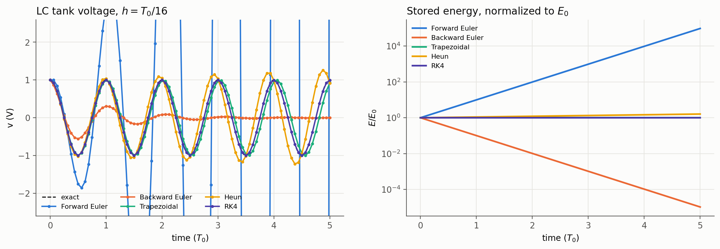
After five periods ($v(5T_0) = 1$ V exactly):
| Method | $v(5T_0)$ | Energy / $E_0$ |
|---|---|---|
| Forward Euler | +28.05 V | 96131 |
| Backward Euler | +0.0003 V | ≈ 0 |
| Trapezoidal | +0.923 V | 1.0000 |
| Heun | +0.912 V | 1.61 |
| RK4 | +0.998 V | 0.996 |
This matches what the stability functions told us. Forward Euler explodes, because $|1 + j\omega_0 h| > 1$ and the energy grows by a fixed factor every step. Backward Euler damps the tank to nothing within five periods. The trapezoidal method keeps the energy exactly, but the waveform slowly drifts in phase, which is why $v(5T_0)$ is off. Heun slowly gains energy, and RK4 is the closest to the exact solution with a tiny bit of damping.
RC Step Response with a Large Step
Now back to our RC circuit from the beginning ($\tau = 10$ ns), but this time we deliberately use a step size $h = 2.5\tau$, which is larger than what Forward Euler can handle:
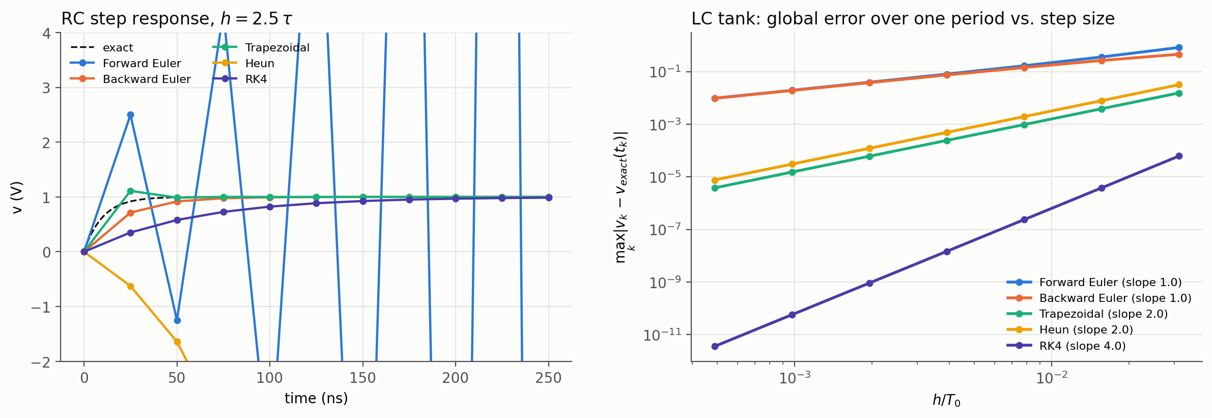
On the left:
- Forward Euler and Heun both diverge, since $h > 2\tau$. After 250 ns, they are at −56.7 V and −127.4 V respectively.
- RK4 is still stable ($2.5 < 2.79$), but it’s inaccurate: after one step it’s at 0.352 V while the exact answer is 0.918 V. Stable doesn’t mean correct.
- Backward Euler settles without any overshoot, just a bit slower than the real circuit.
- Trapezoidal overshoots to 1.111 V on the first step and then rings around the final value: exactly the “trapezoidal ringing” from earlier, since $R(-2.5) = -0.11$ is negative.
On the right, we sweep the step size on the LC tank and plot the maximum error over one period. The slopes on the log-log plot give the order of each method: 1.0 for both Euler methods, 2.0 for trapezoidal and Heun, and 4.0 for RK4, exactly as advertised. Notice also that trapezoidal and Heun share the same slope, but trapezoidal has the smaller error constant.
Back to the Question: Why Is My Extracted Simulation So Slow?
Now we are able to answer the question from the beginning. Circuits are stiff: the time constants of a post-layout netlist span many orders of magnitude, from the slow settling we care about down to the femtosecond-level RC of a tiny parasitic. With an explicit method, the step size would be dictated by that fastest parasitic pole, so explicit methods like RK4 are rarely used in circuit simulators.
Instead, SPICE-family simulators use implicit methods, typically trapezoidal and Gear (BDF2), together with Backward Euler around discontinuities. In Spectre, you can choose among them using the method option of the transient analysis. Implicit methods remove the stability limit, but every time step now requires several Newton-Raphson iterations, and every iteration requires factorizing a matrix whose size grows with the number of nodes. Adding thousands of parasitic nodes therefore makes each time step much more expensive, and the fast parasitic dynamics still force the simulator to take smaller steps to keep the accuracy within tolerance.