We explained some commonly used numerical methods for solving IVP problems in transient simulations in the last post. However, there are sometimes situations where IVP problem doesn’t characterize the system’s behavior adequately.
One such situation is when we are interested in the system’s periodic steady-state behavior rather than its transient response. In these cases, we are more interested in what’s called the Boundary Value Problem (BVP), where the solution is sought over a period with specified boundary conditions rather than initial conditions.
Boundary Value Problem (BVP)
Let’s say you have a switched-capacitor filter, or simply our RC circuit from last time, driven by a 1 GHz clock, and you want to know its steady-state output ripple. With a transient simulation, you would have to start from some initial condition and wait for hundreds of cycles until all the start-up transients die out, and then throw most of the waveform away. What we really want is the waveform of one period after the circuit has settled, and the condition that tells us we’ve settled is that the state at the end of the period comes back to where it started. You have just created a boundary value problem (BVP): instead of specifying the state at one point in time and marching forward, we specify conditions that the solution must satisfy at both ends of an interval.
Mathematically, a two-point BVP can be expressed as:
$$ \frac{d\mathbf{x}(t)}{dt} = \mathbf{f}(\mathbf{x}(t), t), \quad f(t_0) = A, \quad f(t_0 + T) = B $$where $\mathbf{x}(t)$ and $\mathbf{f}(\mathbf{x}(t), t)$ are the same as in the IVP, $T$ is the length of the interval. In the special case of periodic steady-state analysis, the boundary conditions are simply:
$$ f(t_0) = f(t_0 + T) $$meaning that the solution repeats itself after one period.
BVPs are generally more challenging to solve than IVPs because the solution must satisfy conditions at multiple points rather than just an initial condition. We will see how we are going to convert a BVP into an IVP, and use whatever we have learned about IVPs to tackle the problem. However, before that we must understand what are the scenarios that BVP might not have a solution.
Preventing the Butterfly Effect
You probably have heard of the “butterfly effect,” which refers to the sensitive dependence on initial conditions in chaotic systems. Sometimes this can create problems when we would like to find the exact solution.
The Lorenz Attractor Example
One famous butterfly effect example is the Lorenz attractor.
In 1963, Edward Lorenz simplified a model of atmospheric convection down to just three state variables, and arrived at the following system of ODEs:
$$ \begin{align*} \begin{cases} \dot{x} &= \sigma (y - x) \\ \dot{y} &= x (\rho - z) - y \\ \dot{z} &= xy - \beta z \end{cases} \end{align*} $$where $\sigma$, $\rho$ and $\beta$ are positive constants. Lorenz used $\sigma = 10$, $\rho = 28$ and $\beta = 8/3$, which are still the standard values today. In our notation, the state vector is $\mathbf{x} = (x, y, z)^T$, and $\mathbf{f}(\mathbf{x})$ is the right-hand side above.
The system looks innocent: it’s only three equations, the only nonlinear terms are the products $xz$ and $xy$, and there is no randomness anywhere. Yet for these parameter values, every trajectory gets pulled onto a bounded, butterfly-shaped set, called the attractor, and keeps looping around its two “wings” forever, switching between them in a pattern that never repeats.
The butterfly effect shows up when we start two simulations from almost the same point. Let’s integrate the system with the RK4 method from the last post, with $h = 0.005$, from $\mathbf{x}_0 = (1, 1, 1)$ and from a second initial state that differs only by $10^{-8}$ in $x$:
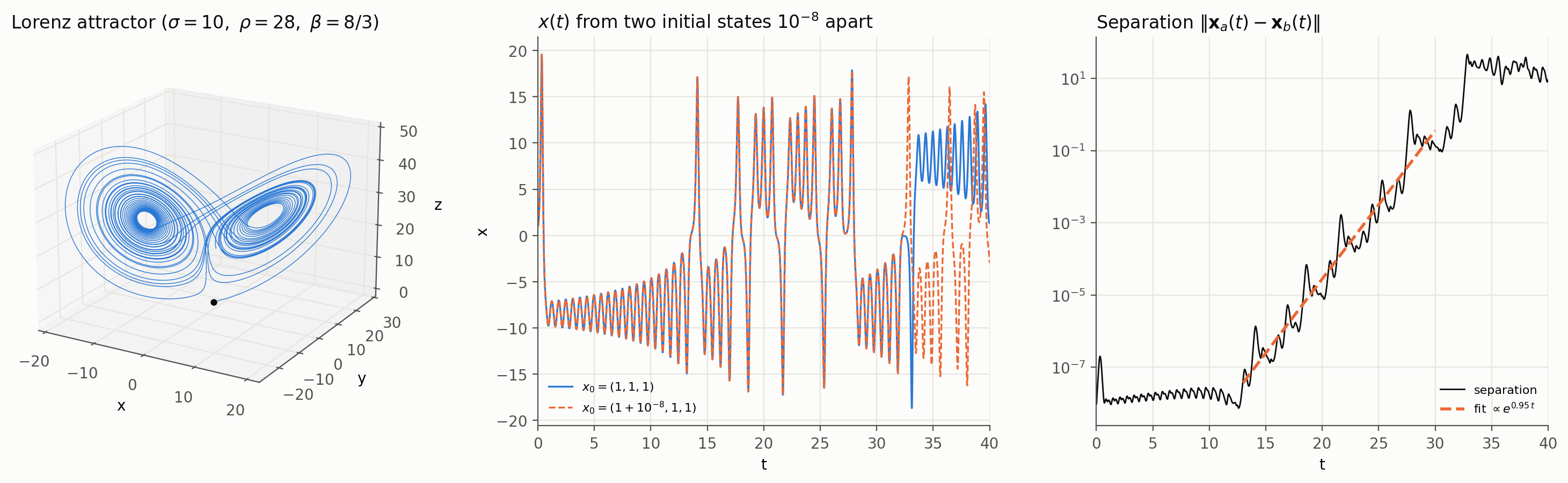
For the first 25 time units, the two waveforms are indistinguishable. Then they suddenly go their separate ways, and after $t \approx 33$ they have nothing to do with each other. On the right, we see why: after an initial settling phase, the separation $\delta(t)$ between the two trajectories grows exponentially,
$$ \delta(t) \approx \delta_0 \, e^{\lambda t} $$until it saturates at the size of the attractor itself. The growth rate $\lambda$ is called the largest Lyapunov exponent. Fitting the growth phase gives a slope of 0.95, and averaging over 1000 time units gives $\lambda \approx 0.90$, i.e. any initial error grows by about $e^{0.9} \approx 2.5\times$ per unit time. A $10^{-8}$ difference, far below anything we could ever measure, reaches order one at $t \approx 28$: about 13 time units of settling, then roughly 20 of exponential growth.
Bear in mind that this is not a numerical artifact: a smaller time step only makes RK4 follow the exact trajectory more closely, and the exact trajectories themselves diverge like this. This is a property of the system, not of the solver.
Continuous Dependence on Initial Conditions
So, is there anything that prevents the butterfly effect? To answer this, let’s go back to the mapping $\psi$ from the IVP, and be a bit more precise about where it lands. For a fixed final time $T$, $\psi$ maps an initial state to a whole trajectory on $[t_0, T]$:
$$ \psi: \mathbb{R}^n \to \mathcal{C}_n[t_0, T], \quad \psi(\mathbf{x}_0)(t) := \mathbf{x}(t, t_0, \mathbf{x}_0) $$where $\mathcal{C}_n[t_0, T]$ is the space of continuous functions from $[t_0, T]$ to $\mathbb{R}^n$. We say $\psi$ is continuous at $\mathbf{x}_0$ if:
$$ \forall \varepsilon > 0, \ \exists \delta > 0 \ \text{ s.t. } \ \|\mathbf{x}_0 - \mathbf{z}_0\| < \delta \Rightarrow \|\psi(\mathbf{x}_0) - \psi(\mathbf{z}_0)\|_\infty < \varepsilon $$On the left, \( \|\cdot\| \) can be any norm on $\mathbb{R}^n$. On the right, the norm is the infinity norm over the whole trajectory:
$$ \|\psi(\mathbf{x}_0) - \psi(\mathbf{z}_0)\|_\infty = \sup_{t_0 \le t \le T} \|\mathbf{x}(t) - \mathbf{z}(t)\| $$Or, in terms of balls:
$$ \mathbf{z}_0 \in B_\delta(\mathbf{x}_0) \Rightarrow \psi(\mathbf{z}_0) \in B_\varepsilon(\psi(\mathbf{x}_0)) $$In plain words: if we start close enough, the worst-case difference between the two trajectories over the entire interval stays bounded by $\varepsilon$. This is exactly what “preventing the butterfly effect” means.
Theorem (Continuous Dependence on Initial Conditions): Consider $\dot{\mathbf{x}} = \mathbf{f}(t, \mathbf{x})$, $\mathbf{x} \in \mathbb{R}^n$, where $\mathbf{f}(t, \mathbf{x})$ satisfies the conditions of the global existence and uniqueness theorem. Fix $T \in [t_0, +\infty)$, and suppose $\mathbf{x}(\cdot)$ and $\mathbf{z}(\cdot)$ are two solutions satisfying
$$ \begin{align*} \dot{\mathbf{x}} &= \mathbf{f}(t, \mathbf{x}), \quad \mathbf{x}(t_0) = \mathbf{x}_0 \\ \dot{\mathbf{z}} &= \mathbf{f}(t, \mathbf{z}), \quad \mathbf{z}(t_0) = \mathbf{z}_0 \end{align*} $$Then $\forall \varepsilon > 0, \ \exists \delta > 0$ such that
$$ \|\mathbf{x}_0 - \mathbf{z}_0\| < \delta \Rightarrow \sup_{t_0 \le t \le T} \|\mathbf{x}(t) - \mathbf{z}(t)\| < \varepsilon $$
Wait, doesn’t the Lorenz attractor contradict this? Not really. The key word is fix $T$: the theorem promises a $\delta$ for every finite interval, but says nothing about how small that $\delta$ has to be. For the Lorenz system, the separation grows like $e^{\lambda t}$, so keeping the trajectories within $\varepsilon$ up to time $T$ requires roughly \( \delta \sim \varepsilon \, e^{-\lambda (T - t_0)} \). Continuity still holds, but $\delta$ shrinks exponentially as the interval gets longer.
Here is why this matters for BVPs. Recall that the periodic steady state is a root of $F(\mathbf{x}_0) = \psi(\mathbf{x}_0)(t_0 + T) - \mathbf{x}_0$. To solve it with Newton’s method, we need the sensitivity of the final state with respect to the initial state, $\partial \psi / \partial \mathbf{x}_0$, which grows like $e^{\lambda T}$ for a chaotic system. Over a long interval, a tiny change in $\mathbf{x}_0$ changes $F$ by an enormous amount, and the problem becomes hopelessly ill-conditioned.
Continuous Dependence on Initial Conditions
We defined function $\psi$ in the last post. As a reminder:
$$ \psi(\mathbf{x}_0)(t) = \mathbf{x}(t) $$where $\mathbf{x}(t)$ is the solution of the initial value problem
$$ \begin{cases} \dot{\mathbf{x}} = \mathbf{f}(\mathbf{x}), \\ \mathbf{x}(t_0) = \mathbf{x}_0. \end{cases} $$To prevent small changes in the initial state from causing large deviations in the solution, we require the system to have continuous dependence on initial conditions. Formally, this means that for any $\epsilon > 0$, there exists a $\delta > 0$ such that if \( \|\mathbf{x}_0 - \mathbf{y}_0\| < \delta \), then
$$ \|\psi(\mathbf{x}_0)(t) - \psi(\mathbf{y}_0)(t)\| < \epsilon \quad \text{for all } t \in [t_0, t_0 + T]. $$Shooting Method
Now we are ready to solve a BVP. Let’s use the following problem as our running example:
$$ \ddot{x} + x = 0, \qquad x(0) = 1, \qquad x(\pi/2) = 2 $$This one has a closed-form solution, so we can check our answers. Every solution of the ODE has the form $x(t) = A\cos t + B\sin t$. From $x(0) = 1$ we get $A = 1$, and from $x(\pi/2) = 2$ we get $B = 2$:
$$ x(t) = \cos t + 2\sin t, \qquad \dot{x}(0) = 2 $$NoteA second-order ODE needs two conditions, but not every choice works. Don’t use $x(\pi)$ as the second condition: every solution with $x(0) = 1$ has $x(\pi) = -1$, so that condition gives either no solution or infinitely many.
Idea
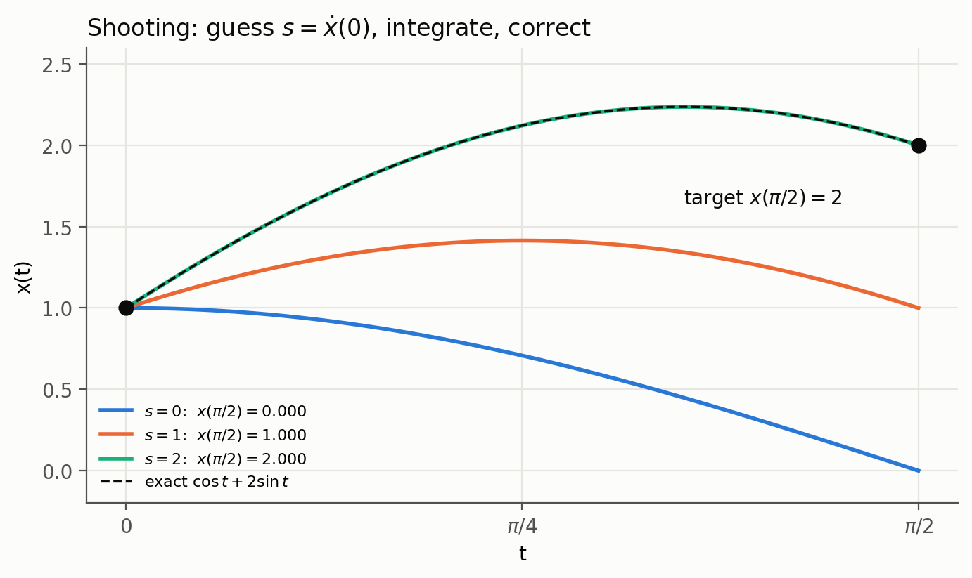
Remember that we promised to convert a BVP into an IVP. The shooting method does exactly that. If we knew the initial slope $s = \dot{x}(0)$, this would just be an IVP, and we know how to solve those. So let’s guess $s$, integrate forward, and see by how much we miss the far boundary:
$$ F(s) = x(\pi/2; s) - 2 $$where $x(\pi/2; s)$ is the solution at $t = \pi/2$ when we start with slope $s$. The BVP is now a root-finding problem: find $s$ such that $F(s) = 0$. Just like aiming a cannon: fire, see where the ball lands, adjust the angle, fire again.
For periodic steady state, the idea is the same, except that the unknown is the whole initial state, and the miss is measured against the initial state itself:
$$ F(\mathbf{x}_0) = \psi(\mathbf{x}_0)(t_0 + T) - \mathbf{x}_0 = 0 $$Steps
Rewrite the problem as a first-order system with $y_1 = x$ and $y_2 = \dot{x}$:
$$ \dot{y}_1 = y_2, \qquad \dot{y}_2 = -y_1, \qquad \mathbf{y}(0) = [1, s]^T $$Guess $s_0 = 0$. Integrating gives $x(\pi/2) = 0$, so $F_0 = -2$.
Guess $s_1 = 1$. Integrating gives $x(\pi/2) = 1$, so $F_1 = -1$.
Secant update:
$$ s_2 = s_1 - F_1 \frac{s_1 - s_0}{F_1 - F_0} = 1 - (-1)\frac{1}{1} = 2 $$$F(2) \approx 0$, so we have converged to $\dot{x}(0) = 2$.
Because the ODE is linear, $F(s)$ is linear in $s$, and the secant method converges in one step. A nonlinear ODE would take a few iterations.
Code
Let’s reuse the RK4 integrator from the last post:
 1T, X0, XT = np.pi / 2, 1.0, 2.0                   # x(0) = 1, x(T) = 2
 2f = lambda y, t: np.array([y[1], -y[0]])          # y = [x, x']
 3
 4def F(s, h=T / 200):
 5    """Integrate with x(0) = 1, x'(0) = s; return the miss at the far boundary."""
 6    t, y = integrate(rk4_step, f, np.array([X0, s]), 0.0, T, h)
 7    return y[-1, 0] - XT
 8
 9def shoot(s0=0.0, s1=1.0, tol=1e-10):
10    F0, F1 = F(s0), F(s1)
11    history = [(s0, F0), (s1, F1)]
12    while abs(F1) > tol:
13        s0, F0, s1 = s1, F1, s1 - F1 * (s1 - s0) / (F1 - F0)   # secant step
14        F1 = F(s1)
15        history.append((s1, F1))
16    return s1, history
Running it, the three guesses give:
| Guess | $s$ | $F(s)$ |
|---|---|---|
| 0 | 0 | −2.000 |
| 1 | 1 | −1.000 |
| 2 | 1.999999999951 | $-1.8 \times 10^{-15}$ |
The remaining $5 \times 10^{-11}$ error in $s$ comes from RK4’s truncation error with $h = T/200$, not from the shooting itself.
Bear in mind that for a nonlinear system with many states, we’d use Newton’s method instead of the secant method, which requires the Jacobian $\partial \psi / \partial \mathbf{x}_0$, the sensitivity of the final state to the initial state. This is exactly where the butterfly effect bites: for a chaotic (or just very sensitive) system, this Jacobian grows exponentially with the interval length.
Harmonic Balance
Idea
The shooting method works in the time domain. Harmonic balance goes the other way: assume the solution is a truncated Fourier series, substitute it into the ODE, and require the coefficient of each harmonic in the residual to vanish. This turns the ODE into a set of algebraic equations for the Fourier coefficients, plus the frequency $\omega$ if it is unknown.
Steps
Ansatz with $N$ harmonics:
$$ x(t) = a_0 + \sum_{k=1}^{N} \left[ a_k \cos(k\omega t) + b_k \sin(k\omega t) \right] $$Substitute. Since $\ddot{x} = -\sum_k (k\omega)^2 [a_k\cos(k\omega t) + b_k\sin(k\omega t)]$, we have
$$ \ddot{x} + x = a_0 + \sum_{k=1}^{N} (1 - k^2\omega^2)\left[a_k\cos(k\omega t) + b_k\sin(k\omega t)\right] $$Balance each harmonic:
- DC: $a_0 = 0$
- $k$-th harmonic: $(1 - k^2\omega^2) a_k = 0$ and $(1 - k^2\omega^2) b_k = 0$
A nonzero solution needs $k\omega = 1$ for some $k$. Taking $k = 1$ gives $\omega = 1$, and every other harmonic vanishes:
$$ x(t) = A\cos t + B\sin t $$Note that the balance fixes the frequency, but not the amplitudes, because the ODE is linear and unforced.
Apply the boundary conditions: $x(0) = A = 1$ and $x(\pi/2) = B = 2$, so
$$ x(t) = \cos t + 2\sin t $$
The result is exact because the true solution happens to be a single harmonic. In a nonlinear ODE, e.g. the Duffing equation $\ddot{x} + x + \varepsilon x^3 = 0$, the harmonics couple to each other ($\cos^3 t$ produces $\cos 3t$), so the balance equations become nonlinear, and $\omega$ depends on the amplitude.
Code
Numerically, we stack the unknowns $[\omega, a_0, \ldots, a_N, b_1, \ldots, b_N]$ into one vector, and solve the harmonic balance equations together with the two boundary conditions. There are more equations than unknowns, so we solve it in the least-squares sense with Gauss-Newton:
 1N = 3                                              # number of harmonics
 2
 3def unpack(p):                                     # p = [w, a0..aN, b1..bN]
 4    return p[0], p[1:N + 2], np.r_[0.0, p[N + 2:]]
 5
 6def x_hb(t, a, b, w):
 7    k = np.arange(N + 1)[:, None]
 8    return (a[:, None] * np.cos(k * w * t) + b[:, None] * np.sin(k * w * t)).sum(0)
 9
10def residual(p):
11    w, a, b = unpack(p)
12    k = np.arange(N + 1)
13    hb = np.r_[(1 - (k * w) ** 2) * a, ((1 - (k * w) ** 2) * b)[1:]]   # each harmonic of x'' + x
14    bc = [x_hb(np.array([0.0]), a, b, w)[0] - X0,                      # boundary conditions
15          x_hb(np.array([T]), a, b, w)[0] - XT]
16    return np.r_[hb, bc]
17
18def gauss_newton(r, p, tol=1e-14, max_iter=100):
19    """Least-squares Newton: p <- p - lstsq(J, r(p)), finite-difference Jacobian."""
20    for it in range(max_iter):
21        rp = r(p)
22        J = np.empty((rp.size, p.size))
23        for j in range(p.size):
24            dp = np.zeros_like(p); dp[j] = 1e-7
25            J[:, j] = (r(p + dp) - rp) / dp[j]
26        step = np.linalg.lstsq(J, rp, rcond=None)[0]
27        p = p - step
28        if np.max(np.abs(step)) < tol:
29            break
30    return p, it + 1
31
32p0 = np.r_[0.9, 0.5 * np.ones(N + 1), 0.5 * np.ones(N)]   # rough initial guess
33p, iters = gauss_newton(residual, p0)
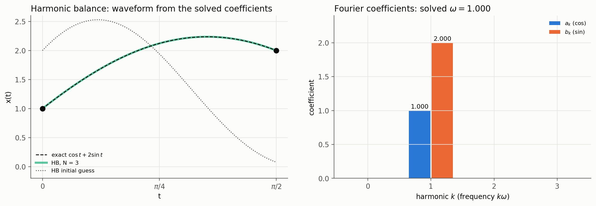
Starting from a rough guess of $\omega = 0.9$ and all coefficients at 0.5, it converges in 8 iterations to $\omega = 1$, $a = [0, 1, 0, 0]$ and $b = [0, 2, 0, 0]$. The 2nd and 3rd harmonics come out as zero, and the reconstructed waveform matches $\cos t + 2\sin t$ to machine precision.
From BVP to Periodic Steady State: Two Practical Scenarios
So far, our example came with two nice boundary conditions handed to us. Real PSS problems are not that kind. When we ask the simulator for the periodic steady state of a circuit, we usually don’t know the state at the start of the period, and for an oscillator we don’t even know how long the period is. Let’s look at how each of these situations is turned into something the shooting method and harmonic balance can solve.
Scenario 1: Driven Circuit, Unknown Initial State
This is the typical case: a circuit driven by a periodic source with a known period $T$, like a clock or an LO. We want the steady state, but we have no idea what the state looks like at the start of a period; that’s exactly what we’re trying to find.
The trick is that periodicity itself replaces the missing initial condition:
$$ \mathbf{x}(t_0 + T) = \mathbf{x}(t_0) $$That’s $n$ equations for the $n$ unknown components of $\mathbf{x}_0 = \mathbf{x}(t_0)$, which is a well-posed problem.
Shooting: we solve $F(\mathbf{x}_0) = \psi(\mathbf{x}_0)(t_0 + T) - \mathbf{x}_0 = 0$ with Newton’s method. Each Newton iteration integrates one period of transient, and the Jacobian is
$$ \frac{\partial F}{\partial \mathbf{x}_0} = \frac{\partial \psi(\mathbf{x}_0)(t_0 + T)}{\partial \mathbf{x}_0} - I $$The first term is the sensitivity of the end-of-period state to the start-of-period state, also known as the monodromy matrix. For a linear circuit, $F$ is linear, and Newton converges in one step.
Harmonic balance: here periodicity comes for free. Every term of a Fourier series with fundamental $\omega = 2\pi/T$ is already $T$-periodic, so there is no initial condition to find at all; we only solve for the coefficients. For a linear circuit, the harmonics don’t even talk to each other, and harmonic balance reduces to an AC analysis at each harmonic: $V_k = Z(jk\omega) I_k$.
Example. Let’s go back to the RC circuit from the last post (\( R = 10\,\text{k}\Omega \), \( C = 1\,\text{pF} \), $\tau = 10$ ns), and drive it with a square-wave current that switches between 0 and 100 µA at 1 GHz. This is the “RC driven by a clock” from the beginning of this post. The capacitor charges during the first half of the period and discharges during the second half, and in steady state the two exponential segments must connect. Solving for the end points gives the closed-form answer:
$$ v_{min} = IR\frac{e^{-a}}{1 + e^{-a}}, \qquad v_{max} = IR\frac{1}{1 + e^{-a}}, \qquad a = \frac{T}{2\tau} $$i.e. $v_{min} = 487.503$ mV, $v_{max} = 512.497$ mV, a ripple of 24.99 mV around 500 mV.
The numbers:
- Plain transient: starting from 0 V, it takes 131 periods before the waveform settles within 1 µV of the steady state, since the settling is governed by $\tau = 10T$.
- Shooting: Newton converges after integrating only 6 periods in total (including the extra integrations for the finite-difference Jacobian), and lands on the exact $v_{min}$ to within $2 \times 10^{-15}$ V.
- Harmonic balance: the square wave has sharp edges, so the waveform has a corner at every edge, and the Fourier coefficients decay slowly. The worst-case error over the period is 2.37 mV with 1 harmonic, 0.84 mV with 5, 0.195 mV with 25, and still 0.050 mV with 101 harmonics.
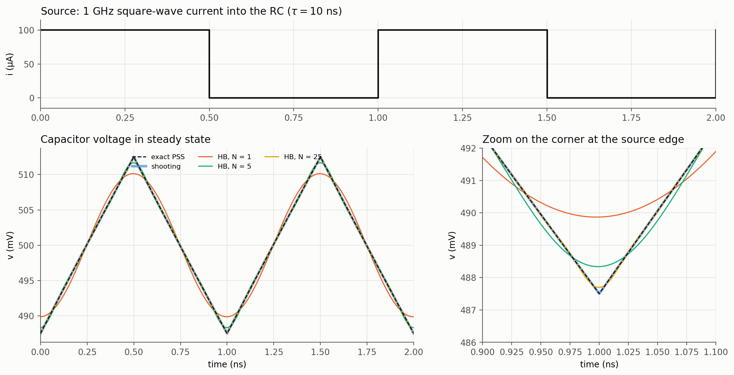
Note that the capacitor voltage itself is not a square wave: with $\tau = 10T$, the RC integrates the square-wave current into a triangle with 25 mV of ripple. The trouble for harmonic balance is the sharp corner at every source edge, which the zoom on the right shows: with 1 harmonic the corner is badly rounded off, with 5 it’s better, and only around 25 harmonics does it follow the exact solution closely.
WarningThe source edge at $T/2$ is a discontinuity, and an RK4 step that straddles it applies the wrong current for part of the step. In my first attempt, this alone left an error of about 0.5 mV in the steady state. The fix is what every circuit simulator does with breakpoints: end a time step exactly at the edge, and restart the integration from there.
Scenario 2: Autonomous Circuit, Unknown Period
Now consider an oscillator: a ring oscillator, an LC VCO, or anything without a periodic input. Two new problems show up:
- The period $T$ is unknown. It’s set by the circuit itself, so $T$ becomes an extra unknown, and we now have $n + 1$ unknowns but only $n$ periodicity equations.
- The phase is arbitrary. Since nothing drives the circuit, any time-shifted copy of a periodic solution is also a periodic solution, so there are infinitely many of them.
Both problems are solved together by adding one phase condition, which pins down where the period starts. That gives $n + 1$ equations for $n + 1$ unknowns. On top of that, the DC operating point $\mathbf{x}(t) = \mathbf{x}_{DC}$ trivially satisfies periodicity for any $T$. This is why oscillator PSS needs a good initial guess, and why simulators typically run a short transient first to get the oscillation going.
- Shooting: the unknowns are $(\mathbf{x}_0, T)$. A convenient phase condition is to start the period at a peak of one state variable, i.e. $\dot{x}_j(t_0) = 0$.
- Harmonic balance: the unknowns are the Fourier coefficients plus $\omega$. A convenient phase condition is to set the sine coefficient of the fundamental of one variable to zero, $b_1 = 0$, which lines up its fundamental with a cosine.
Example. The classic model of an oscillator is the Van der Pol oscillator:
$$ \ddot{x} - \mu (1 - x^2) \dot{x} + x = 0 $$which is (in normalized units) an LC tank in parallel with a nonlinear conductance $-g_1 v + g_3 v^3$, a crude model of a cross-coupled pair: negative resistance at small amplitude to start the oscillation, and compression at large amplitude to limit it. We take $\mu = 1$, where there is no closed-form solution.
For shooting, the phase condition $\dot{x}(0) = 0$ means $x(0) = A$ is the amplitude, and the unknowns are just $[A, T]$:
1def shoot_vdp(A0=1.5, T0=2 * np.pi):
2    """Unknowns [A, T]; phase condition x'(0) = 0, i.e. start the period at a peak x(0) = A."""
3    def F(p):
4        A, T = p
5        y_end = integrate(rk4_step, f_vdp, np.array([A, 0.0]), 0.0, T, T / N_STEPS)[1][-1]
6        return np.array([y_end[0] - A, y_end[1] - 0.0])
7    return newton(F, np.array([A0, T0]))
Starting from a guess of $A = 1.5$ and $T = 2\pi$, it converges to $A = 2.0086$ and $T = 6.6633$, which matches the known period for $\mu = 1$.
For harmonic balance, the nonlinear term $x^2 \dot{x}$ is awkward to expand by hand. Instead, we evaluate the residual at sample points in the time domain, and project it back onto the harmonics with a Fourier transform. This time-domain/frequency-domain round trip is also how harmonic balance simulators handle nonlinear devices. The results:
| Harmonics $N$ | Period $T$ | Error vs. shooting |
|---|---|---|
| 1 | 6.283185 | $3.8 \times 10^{-1}$ |
| 3 | 6.665495 | $2.2 \times 10^{-3}$ |
| 5 | 6.663382 | $9.5 \times 10^{-5}$ |
| 7 | 6.663287 | $1.8 \times 10^{-7}$ |
| 11 | 6.663287 | $1.1 \times 10^{-9}$ |
With a single harmonic, harmonic balance gives exactly $T = 2\pi$ and an amplitude of 2. This is the describing function result that you may remember from analyzing oscillators by hand: it assumes the waveform is a pure sinusoid, and therefore misses the frequency shift caused by the harmonics. With more harmonics, the error drops very quickly, because the waveform is smooth.
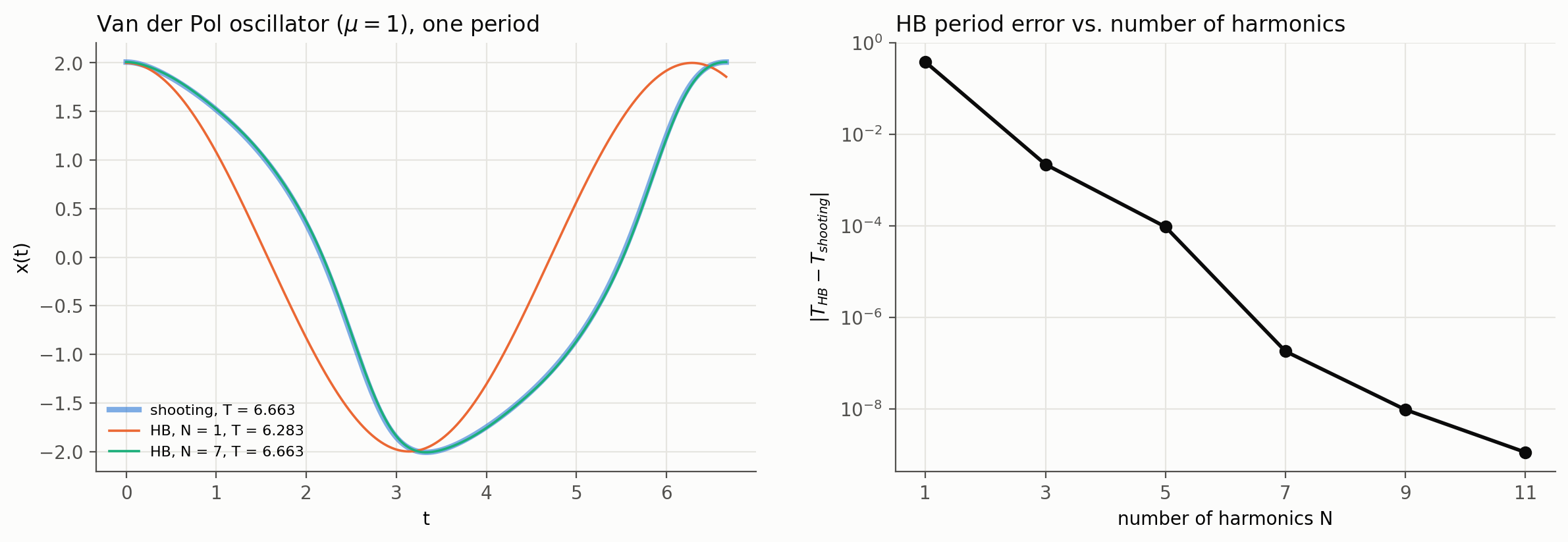
Note that the two methods use different phase conditions, so I aligned the HB waveforms to the peak at $t = 0$ in the left plot.
Summary
| Driven circuit | Autonomous circuit | |
|---|---|---|
| Known | Period $T$ | Nothing |
| Unknowns | $\mathbf{x}_0$ | $\mathbf{x}_0$ and $T$ |
| Equations | Periodicity ($n$) | Periodicity ($n$) + phase condition ($1$) |
| Shooting | Newton on $\psi(\mathbf{x}_0)(T) - \mathbf{x}_0$ | Same, with $T$ as an unknown and e.g. $\dot{x}_j(0) = 0$ |
| Harmonic balance | Coefficients at known $\omega$ | Coefficients and $\omega$, with e.g. $b_1 = 0$ |
The two examples also show the trade-off between the two methods nicely. The switching waveform of the driven RC is exact with shooting, but with harmonic balance the error only falls like $1/N$: going from 25 to 101 harmonics buys just a 4× improvement. The smooth waveform of the Van der Pol oscillator is captured to $10^{-9}$ with 11 harmonics.