Last year when I was taping out Kodiak, my colleague Daniel during my design review asked me, “hey Di, all these PLL designs look great, but one thing that concerns me is that you are using ideal voltage source for your reference clock. Is there a way that you can model the phase noise of the reference?”

Indeed that was a very valuable question, and I didn’t have a good answer for that back then. After some research and experimentation, I grasped the key concepts + techniques to properly model the phase noise of a square wave in time domain. I have kept forgetting how to do this properly since then, and today I want to have this well-documented.

The Physical Meaning of dBc/Hz

[dBc/Hz] is the unit for phase noise, but what does it mean?

Let’s use a sine wave as an example. Suppose our carrier signal is given by:

For simplicity, let’s assume the amplitude is constant and equal to 1.

Here, \( \phi(t) \) represents the phase noise, which is a small deviation from the ideal phase \( \omega t \). Now, given the phase noise is small, we can use trigonometric identities, and apply Taylor series expansion, and discard higher-order terms:

We realize that by multiplying with the signal \( \cos (\omega t) \), we preserved the phase deviation’s power. The other way to look at this is that by convolution theorem, the spectrum of the product is the convolution of the spectra of the individual signals. Given the PSD of both sine and cosine waves are two delta functions at \( \pm \omega \), the total power of the product remains the same as the power of the phase deviation.

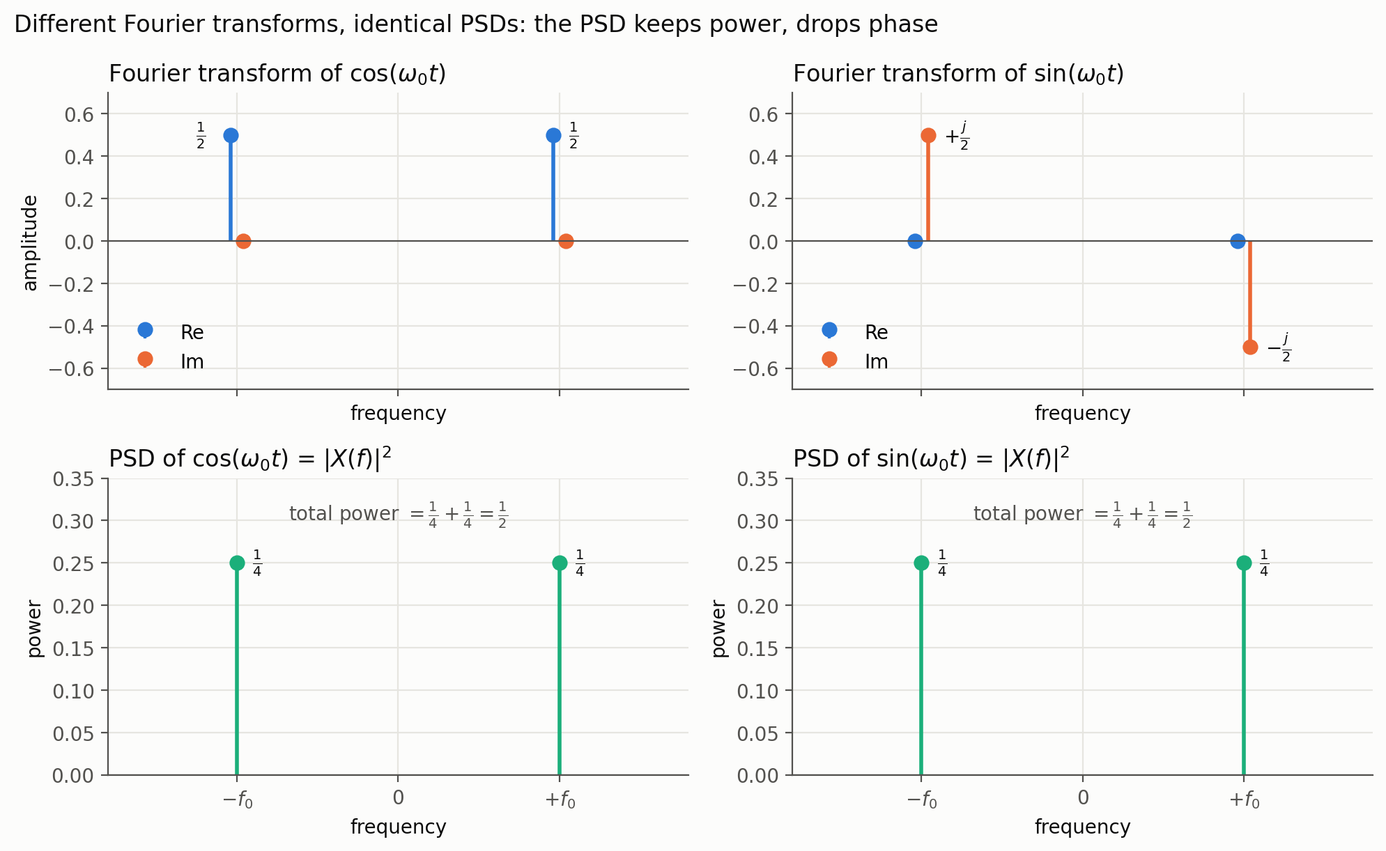
Phase noise is therefore defined as the noise power divided by the carrier power.

The power of a sine wave is $ \frac{1}{2} $; and if we look at the power of the second signal:

Assuming \( \phi(t) \) is a zero-mean stationary process and independent of the carrier, we have:

Therefore, the phase noise in linear scale is:

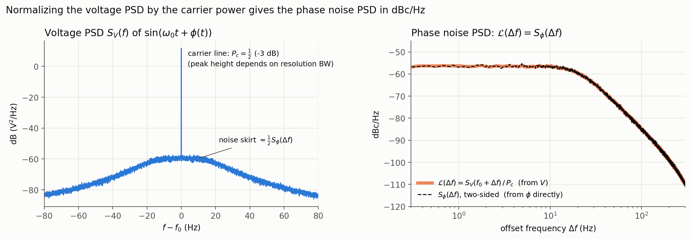
Bear in mind that both $ P_{\text{phase deviation}} $ and $ P_{\text{carrier}} $ have units of “watts”, but the divided quantity $ PN $ is dimensionless. However it just happens that for this small phase noise approximation, the value of phase noise equals the power of the phase deviation itself.

This approximation applies to square waves, or any periodic waveform because we can always decompose the waveform into a sum of sinusoidal components using Fourier series, and the phase noise analysis can be applied to each sinusoidal component individually. For example, for a square wave:

⚠️ Warning

The small phase noise approximation assumes that the phase deviation \( \phi(t) \) is much smaller than 1 radian. If the phase noise is large, such approximation doesn’t hold and you’ll have to use “phase diffusion constant” to characterize the “Lorentzian Spectrum”. This is discussed in Prof. Behzad Razavi’s CMOS PLL book, chapter 2.2.3.

The Shape of a Typical Oscillator Phase Noise

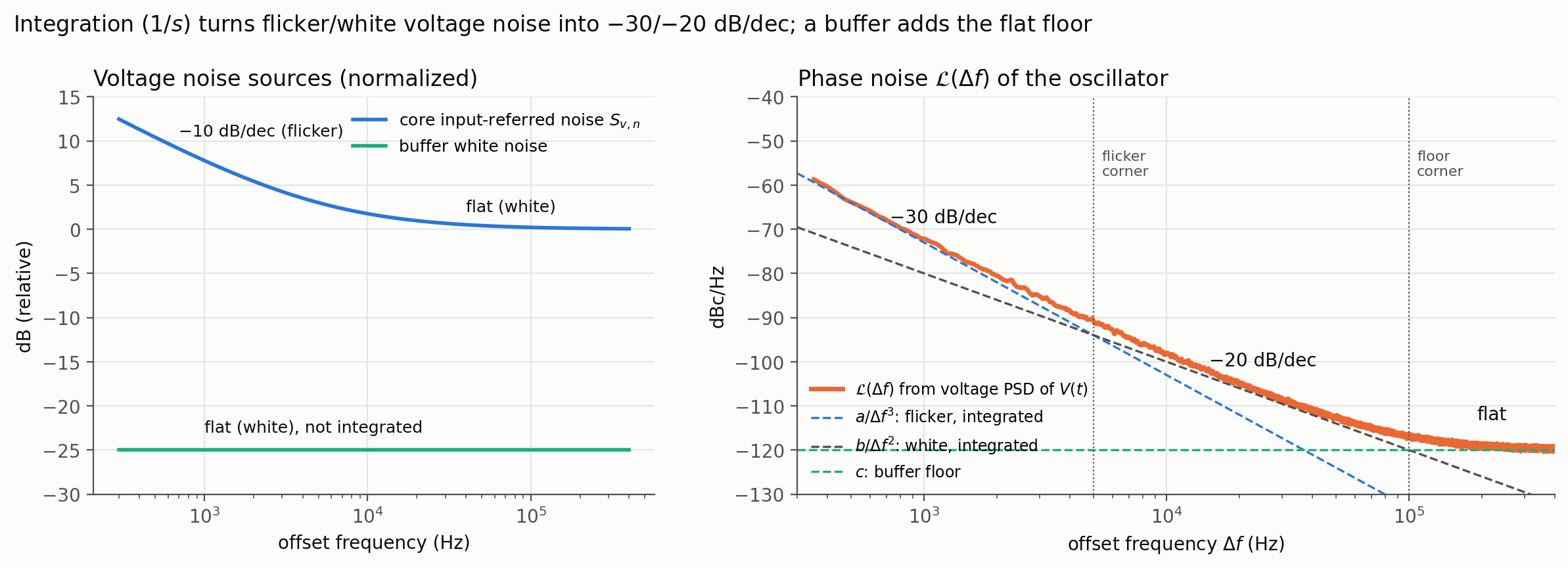
The phase noise of an oscillator is such that it begins with a -30dB/decade slope, followed by a -20dB/decade slope at higher offset frequencies, and finally flattens.

The reason for this behavior lies in the different noise sources affecting the oscillator. If we think about the input-referred noise of the oscillator, it behaves like any other voltage noise source, including flicker noise and white noise.

We know a VCO performs voltage to phase integration – it’s like a $1/s$ operation in the frequency domain. Given flicker noise has -10dB/decade roll-off and white noise is flat, the resulting spectrum therefore exhibits a -30dB/decade slope at low offset frequencies (due to flicker noise) and a -20dB/decade slope at higher offset frequencies (due to white noise), before eventually flattening out.

📝 Note

“performs voltage to phase integration” is a heavily hand-wavy description. The correct way to describe this is that given an oscillator is a time-varying system, it shifts the input-referred voltage noise to the oscillator’s band as an offset, then performs an integration.

The reason for flattening out is due to the white noise of other non-integrating participants in the circuit, for example a clock buffer. Instead of integrating, it simply converts its own voltage noise directly into phase noise because any clock has a non-zero rise and fall time, and the voltage to phase conversion is approximately linear. Usually the sharper the edge is, the smaller the conversion from voltage noise to phase noise is.

⚠️ Warning

As discussed above, small angle approximation usually holds; however if we keep reducing the offset frequency towards very low values, the phase deviation may become large enough that the approximation no longer holds. A general rule of thumb of the lower offset frequency depends on how long we want to observe the system, and whether the system itself can tolerate low-frequency drifts. For example, we don’t care too much about offset frequency of 1e-6 Hz, because that means the observation time can be 11 days.

Modeling the Oscillator Phase Noise

There are a couple of useful Verilog-A functions in Cadence’s Spectre simulator for modeling oscillator phase noise.

1. idt function is perhaps the most commonly used function if the frequency of the oscillator is not a constant. Like the name suggests, it performs an integration over time, starting from an initial condition ic:

2. idtmod function is the circular integrator. Given that usually we only care about the phase within a $2\pi$ range, this function performs integration modulo a given modulus (here $2\pi$):

Bear in mind that both of these perform actions in the time domain, but they do have effect in frequency domain as well, as we will see later.

3. white_noise function is used to generate white noise in the time domain. It does exactly the computation that I described in another post psd to noise conversion. By providing a power spectral density (PSD) value, it generates a corresponding white noise time series.

4. flicker_noise function is used to color a white noise profile. The first argument is the PSD value at 1Hz, and the second argument controls the roll-off of the flicker noise (typically $1/f$).

Now if we combine these two together, we can generate a voltage noise time series like:

1

white_noise(1e-12) + flicker_noise(1e-12, 1)

which corresponds to

Now, we can use idtmod to characterize the phase of an oscillator:

1
2
3

f = 1e9; // example frequency of 1 GHz
omega = 2 * `M_PI * f;
phase = idtmod(omega, 0, 2 * `M_PI);

Here is the interesting part: how are we able to model phase noise here? The trick is to keep using idtmod function, since it does exactly the integration that we just talked about. But here is the question: how are we setting the white noise PSD and flicker noise PSD value?

Our conclusion just now is that the phase noise of an oscillator is, in value, equal to the power of phase deviation. Therefore, if we would like to get a -130 dBc/Hz phase noise at 100 MHz offset, we have the following equation:

⚠️ Warning

Please note that the \( 1/(2\pi f) \) factor comes from the fact that we are doing another integration to have an additional -20dB/dec roll-off, and an integration has a transfer function of \( 1/s = 1/(j 2\pi f) \) in the frequency domain.

Therefore we are able to calculate the required white noise PSD value for the desired phase noise level:

Likewise for flicker noise of -15 dBc/Hz at 10 kHz offset:

Finally, if we want to model the flat phase noise of -150 dBc/Hz, it’s more straightforward:

⚠️ Warning

Straightforward as it seems, this can actually be the most tricky part in simulation, because we always have to set f_max in our testbench. Usually the f_max is given by the Nyquist frequency of the oscillator. However sometimes there are multiple clock sources in the simulation testbench, and that’s where we want to be careful.

For example, if we are simulating a PLL of 8GHz with 100MHz noisy reference with 4GHz f_max, the 50 MHz - 4 GHz phase noise of the reference will be aliased to baseband and raise the noise floor of the reference phase noise. This is not a problem for -20dB/dec and -30dB/dec slopes since they decay quickly and contribute to almost nothing at lower frequencies.

In this case, we’ll have to use a filter function to limit the reference phase noise. This can be done via the laplace_nd(V(in), num, den) Verilog-A function.

In summary, here is the example code snippet that models the white, flicker, and flat phase noise of a 1 GHz oscillator using Verilog-A:

 1
 2
 3
 4
 5
 6
 7
 8
 9
10
11
12
13

S_white_100MHz = -130;
S_flicker_10kHz = -15;
S_flat = -150;

S_white_coefficient = (2 * `M_PI * 100e6)**2 * 10**(S_white_100MHz / 10);
S_flicker_coefficient = (2 * `M_PI)**2 * (10e3)**3 * 10**(S_flicker_10kHz / 10);
S_flat_coefficient = 10**(S_flat / 10);

osc_freq = 1e9; // 1 GHz oscillator frequency

phase = idtmod(2 * `M_PI * osc_freq, 0, 2 * `M_PI)
        + idt(white_noise(S_white_coefficient) + flicker_noise(S_flicker_coefficient, 1))
        + white_noise(S_flat_coefficient);

Trick: Handling Large Noise Coefficients

Suppose you have read this far and tried to implement the phase noise model in your own Verilog-A code. However, the Spectre simulator might yell at you saying the simulation has failed due to the following reason:

1

ERROR: (SPECTRE-16384) Simulation failed due to V exceeds the blowup limit (1GV). 

This error occurs because of the two formulae we used earlier:

If we try to directly calculate how large these two numbers are:

The flicker noise coefficient is extremely large, causing the simulator to directly fail.

To mitigate this issue, we can normalize the noise coefficients or use a scaling factor to bring them within a manageable range for the simulator, and we scale it back later.

 1
 2
 3
 4
 5
 6
 7
 8
 9
10
11
12
13
14
15
16
17
18
19
20

S_white_100MHz = -130;
S_flicker_10kHz = -15;
S_flat = -150;

noise_scale_factor = 1e6;

S_white_coefficient = (2 * `M_PI * 100e6)**2 * 10**(S_white_100MHz / 10) / noise_scale_factor**2;
S_flicker_coefficient = (2 * `M_PI)**2 * (10e3)**3 * 10**(S_flicker_10kHz / 10) / noise_scale_factor**2;
S_flat_coefficient = 10**(S_flat / 10);

osc_freq = 1e9; // 1 GHz oscillator frequency

real_noise_integ = white_noise(S_white_coefficient) + flicker_noise(S_flicker_coefficient, 1);

// phase accumulation: integrate the scaled-down noise, then scale it back up
phase = idtmod(2 * `M_PI * osc_freq, 0, 2 * `M_PI)
        + noise_scale_factor * idtmod(real_noise_integ, 0, 2 * `M_PI / noise_scale_factor)
        + white_noise(S_flat_coefficient);
steps_per_cycle = 100; // example value, adjust as needed
$bound_step(1.0 / osc_freq / steps_per_cycle);

One last note is that $bound_step should be chosen carefully to ensure accurate simulation of the phase noise, especially when dealing with high-frequency oscillators and scaled noise coefficients.

PN Calculator Function in ADE-XL

In another post 相位噪声与抖动的关系 we talked about how to convert a jitter sequence to phase noise. Sometimes writing this in Python is tedious; luckily ADE-XL provides a PN function which is convenient.

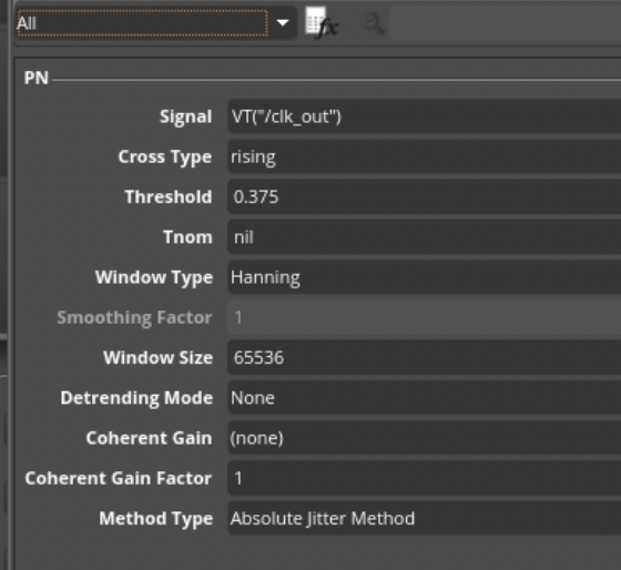
We can use this to verify whether our phase noise model in Spectre matches the expected phase noise calculated from the jitter sequence.

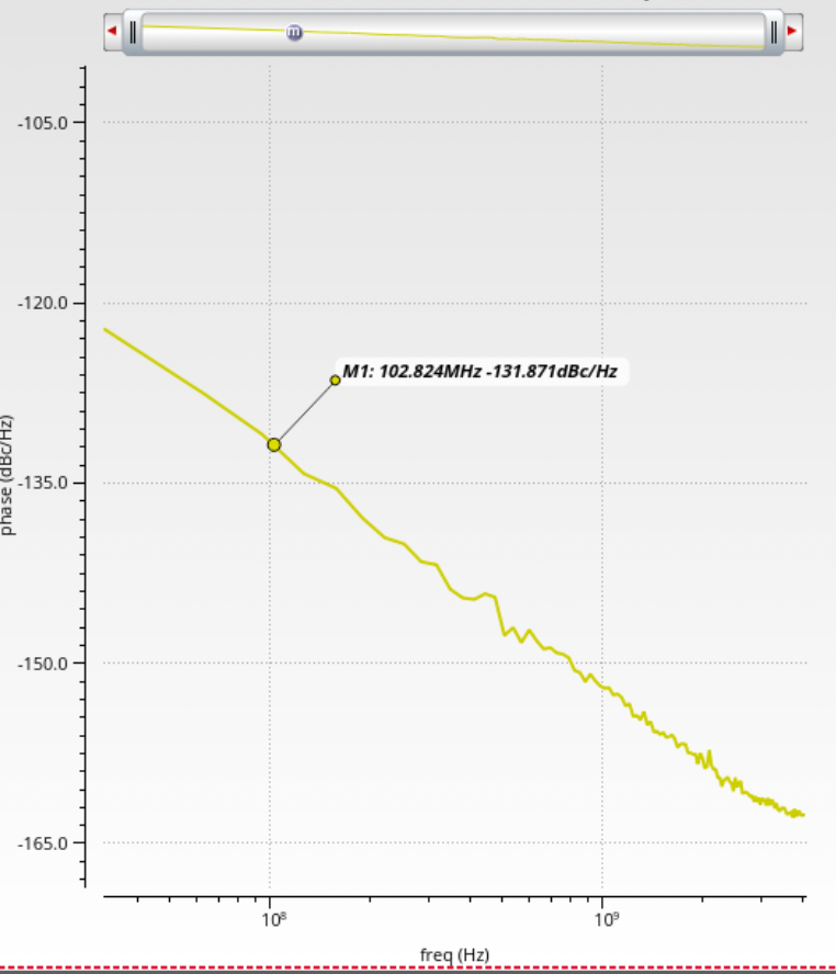
In this example, we use a -130 dBc/Hz white noise coefficient for the 100 MHz offset, and we managed to achieve a good match between the simulated phase noise in Spectre and the expected phase noise calculated from the jitter sequence using the PN function in ADE-XL.