In another post 相位噪声与抖动的关系 we talked about the way to convert a time-domain signal to its frequency-domain representation, which is called Power Spectral Density (PSD). This can be as simple as a Fourier Transform.
However, if we have a PSD, how can we convert it back to a time-domain signal?
A common impression is that integrating the PSD to recover the noise’s standard deviation is wrong, on the grounds that a Gaussian process is white and therefore has a flat PSD. Both halves of that deserve a closer look.
Two claims worth separating
The instinct behind that impression is sound, but it bundles two separate claims — and they do not fare equally well.
Claim 1: “integrating the PSD gives you $\sigma$.” This one is true, and it is true far more generally than people expect. For any wide-sense-stationary process,
$$\sigma^2 = \int_0^{\infty} S_x(f)\,df$$This is the Wiener–Khinchin theorem evaluated at zero lag. It requires neither whiteness nor Gaussianity. It holds for flicker noise, for a random walk, for a narrow bandpass process — for all of them exactly.
Claim 2: “a Gaussian process is a white stationary process with flat PSD.” This one is false. “Gaussian” and “white” are independent properties describing different things:
| what it means | what it describes | |
|---|---|---|
| Gaussian | the amplitude at each instant is normally distributed | the marginal distribution |
| White | samples are mutually uncorrelated; the PSD is flat | the correlation structure |
Pass white Gaussian noise through any linear filter and it remains exactly Gaussian — linear combinations of jointly Gaussian variables are Gaussian — while its PSD becomes arbitrarily colored. So assuming the noise is Gaussian tells you nothing whatsoever about the shape of its spectrum.
So what is the real caution? Not that the integral is wrong, but that it is lossy. The map $S_x(f) \mapsto \sigma$ is many-to-one: infinitely many different spectra integrate to the same $\sigma$. Collapsing a whole function into a single number discards how the power is distributed across frequency — and that distribution, not the total, is what governs how the noise behaves in time.
Four processes, one standard deviation
To make this concrete, here are four Gaussian processes constructed to have identical $\sigma = 1$ but very different spectra: white, $1/f$ flicker, $1/f^2$ random walk, and a 40–60 kHz bandpass process.
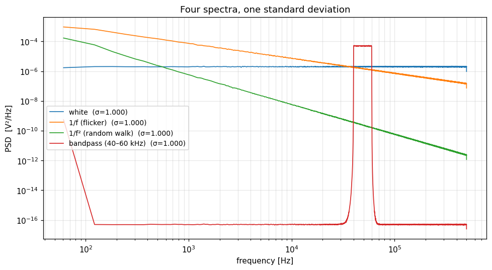
Roughly eight decades of spread in PSD at low frequency — and every one of these curves integrates to the same total power, $\sigma^2 = 1$. If $\sigma$ were a sufficient description of a noise process, these would be interchangeable.
They are not:
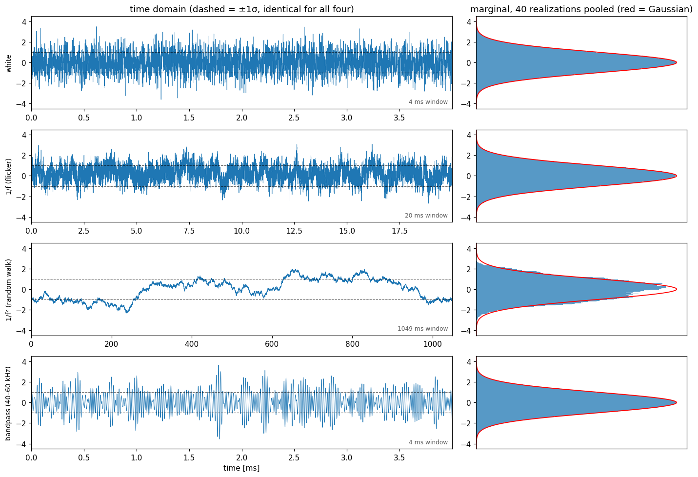
Every histogram on the right matches the same Gaussian curve — all four processes really are Gaussian with $\sigma = 1$. But on the left, the white process rattles between its bounds every sample; the $1/f^2$ process wanders so slowly that a 4 ms window would show nothing but a flat line (it needs a full second to reveal its character); and the bandpass process is a visible 50 kHz burst. Their correlation times differ by more than four orders of magnitude, from 1 sample to roughly 47,000. A single $\sigma$ cannot tell these apart.
Why this matters in practice
In circuit work you rarely care about total integrated noise. You care about noise in a band, because the downstream system only responds to part of the spectrum. Splitting the same four processes by decade — each still at $\sigma = 1$ overall — shows how differently they contribute:
| process | 100 Hz–1 kHz | 1–10 kHz | 10–100 kHz | 100–500 kHz |
|---|---|---|---|---|
| white | 0.042 | 0.134 | 0.424 | 0.894 |
| 1/f (flicker) | 0.409 | 0.409 | 0.409 | 0.342 |
| 1/f² (random walk) | 0.072 | 0.023 | 0.007 | 0.002 |
| bandpass (40–60 kHz) | 0.000 | 0.000 | 1.000 | 0.000 |
Identical totals, completely different band-by-band contributions. This is exactly why a phase-noise or jitter specification is meaningless without its integration limits: integrating $\mathcal{L}(f)$ over different offset ranges yields entirely different jitter numbers from the same device.
One more practical trap, visible only when you compute this numerically: your spectral estimator’s resolution
matters. Welch’s method segments the record, so its lowest resolvable frequency is $f_s/\texttt{nperseg}$, and
any power below that bin is simply never counted. For a $1/f^2$ spectrum, where nearly all the power sits at the
lowest frequencies, this loses most of the variance — the integral comes back as 0.009 instead of 1.0 at
nperseg=8192. That is a measurement artifact, not a failure of Parseval, and it is very likely the origin of
the folklore that “you can’t integrate a PSD to get $\sigma$.”
Going the other way: building a time-domain vector from a PSD
Everything so far has been about what $\sigma$ loses. The constructive counterpart is that the PSD itself loses much less — given $S_x(f)$ you can synthesize a time-domain realization and FFT it straight back to the spectrum you started from. Take a realistic composite of flicker noise over a white floor:
$$S_x(f) = \frac{10^{-12}}{f} + 10^{-16}\ \ \mathrm{V^2/Hz}$$The recipe is short. Set each bin’s magnitude from the target PSD, \(|X_k| = \sqrt{S(f_k)\,\Delta f}\cdot N/\sqrt2\); give each bin an independent uniform random phase; force the spectrum Hermitian so the inverse transform is real (zero the DC bin for zero mean, keep the Nyquist bin real); then inverse-FFT.
1S    = S_target(f)
2mag  = np.sqrt(S * df * N**2 / 2)         # magnitude from the PSD
3ph   = rng.uniform(0, 2*np.pi, f.size)    # phase the PSD never carried
4X    = mag * np.exp(1j*ph)
5X[0], X[-1] = 0, np.abs(X[-1])            # zero mean; real Nyquist bin
6x    = np.fft.irfft(X, n=N)
Here is the vector that comes out — the full record on top, then the same data zoomed in by successive decades, and finally two more realizations drawn with different random phase from the identical PSD:
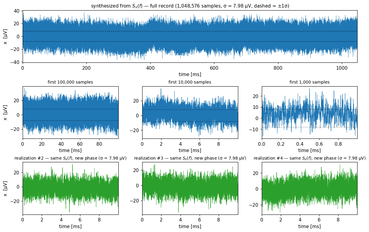
The slow wander across the top panel is the flicker term; the zooms show the self-similar texture $1/f$ noise is known for, looking statistically much the same at 100 ms, 10 ms, and 1 ms. The bottom row is the important one: three waveforms that are visibly different sample by sample, yet share one PSD and one $\sigma$ to the last digit.
FFT that vector back and the recovered spectrum lands on the target across four decades, flicker knee included:
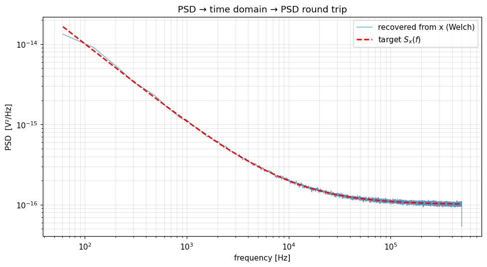
The variance check is exact. Summing $|X_k|^2$ over the coefficients we actually set predicts $\sigma = 7.984169613\times10^{-6}$ V, and the synthesized vector measures $\sigma = 7.984169613\times10^{-6}$ V — agreement to machine precision. Parseval is not approximately true here; it is identically true.
Worth noting what that exactness exposes: computing the same $\sigma$ with np.trapezoid(S, f) comes out 0.39%
low. That is not a flaw in the theorem but quadrature error — $1/f$ varies steeply across the first few bins of a
linear frequency grid, and a trapezoid rule cannot follow it. Real phase-noise data is usually tabulated on a
log grid for exactly this reason, and integrating it naively is another quiet way to get a wrong jitter number.
The asymmetry is the point. Going from PSD to time domain required inventing something the PSD never carried — the phase of every bin. Different phase draws produce completely different-looking waveforms that share one PSD, which is why you can never recover the original waveform from a spectrum, only a statistically equivalent one. Going from time domain to $\sigma$ then discards far more, collapsing an entire function to a single number:
$$\underbrace{x(t)}_{\text{magnitude + phase}} \;\longrightarrow\; \underbrace{S_x(f)}_{\text{magnitude only}} \;\longrightarrow\; \underbrace{\sigma}_{\text{one number}}$$Each arrow is lossy, and the second is by far the more destructive of the two.