We know a jitter is a random variable in time, the next question we would like to ask is how are we going to quantify it.
Histogram Method, Peak-to-Peak, Peak, and RMS
A reasonable first try it to plot the histogram of the jitter samples. Let’s say we send an imperfect clock signal to a high-speed real-time oscilloscope and compare the rising edges of the clock signal to a reference clock. Assume the reference clock is sufficiently clean, that is, the relative jitter between these two clocks construct a sufficiently accurate representation of the absolute jitter sequence, then we collect all deviations of the riging edges to plot a histogram:
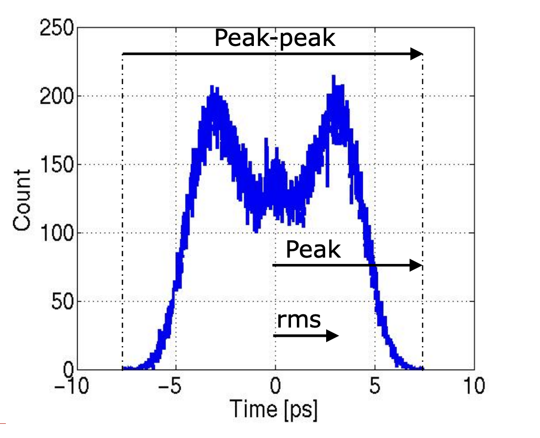
We are able to quantify the jitter, using one number, through the following ways:
- Peak-to-Peak: the maximum difference between the most positive and most negative jitter samples.
- Peak: the maximum absolute value of the jitter samples.
- root-mean-square (RMS): the square root of the average of the squares of the jitter samples.
There are a few pros/cons with each of the above methods:
- peak-to-peak / peak
- easy to calculate
- result is dependent on the length of the measurement.
- Let’s say the jitter source is from an open loop oscillator, which across time has a tendency to increase the absolute jitter. Therefore the peak-to-peak value increases with time, and the longer we measure, the larger the peak-to-peak value.
- RMS
- also easy
- result does not depend on the length of the measurement, as long as we have enough samples to represent the jitter distribution.
- applicable only to Gaussian random variables
- However, if the jitter is bounded within a certain range, then RMS is probably not a good measure compared to the peak-to-peak value, which is able to tell us the worst-case outlier.
Jitter Boundedness
We can see that peak works better for bounded jitter and rms works better for unbounded jitter. What are some examples of these?
Ideal Eye Diagram
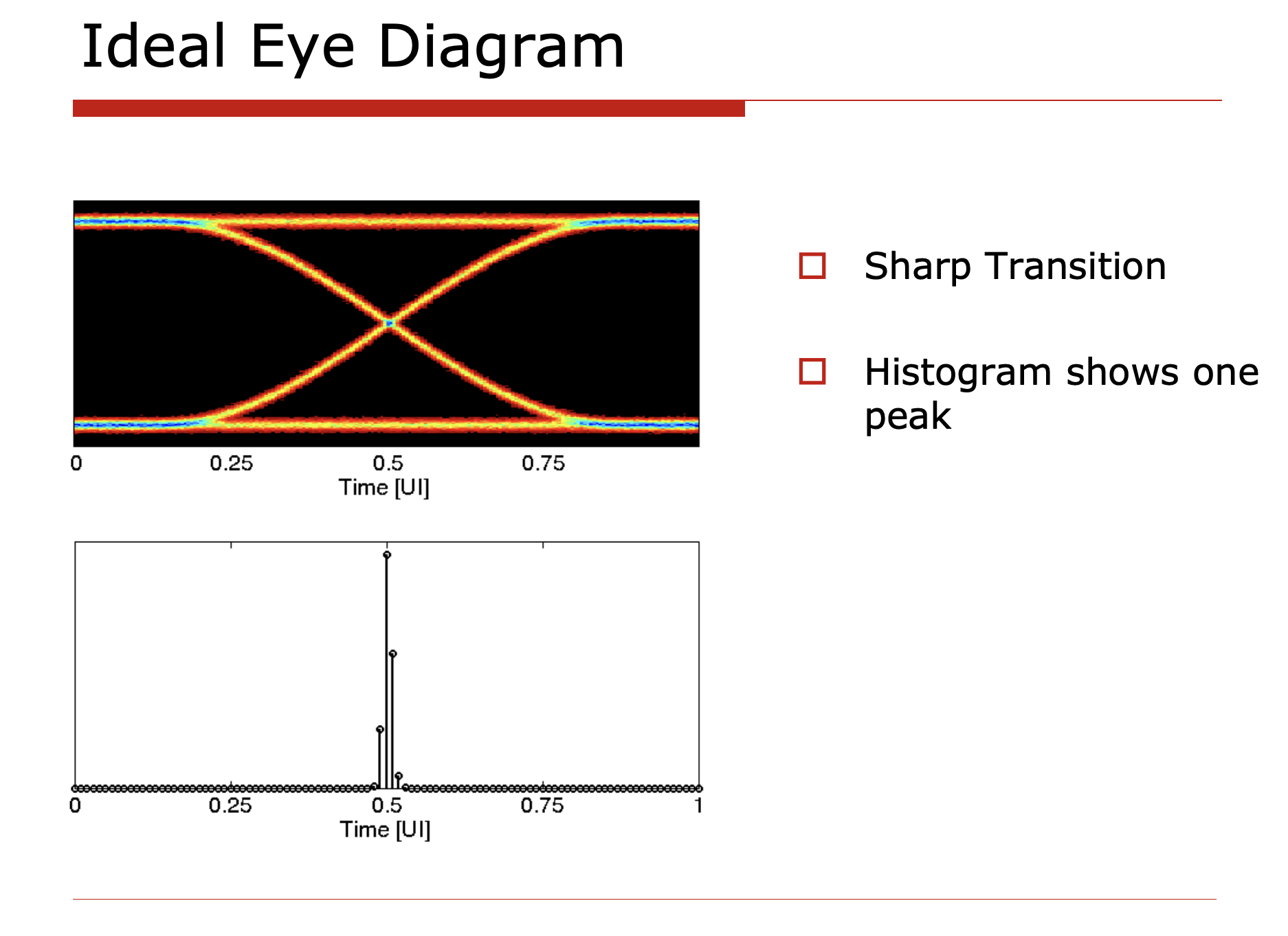
The ideal eye diagram has no jitter at all. All clock edges are perfectly aligned with the reference clock.
The histogram looks like a Dirac delta function.
Random Jitter
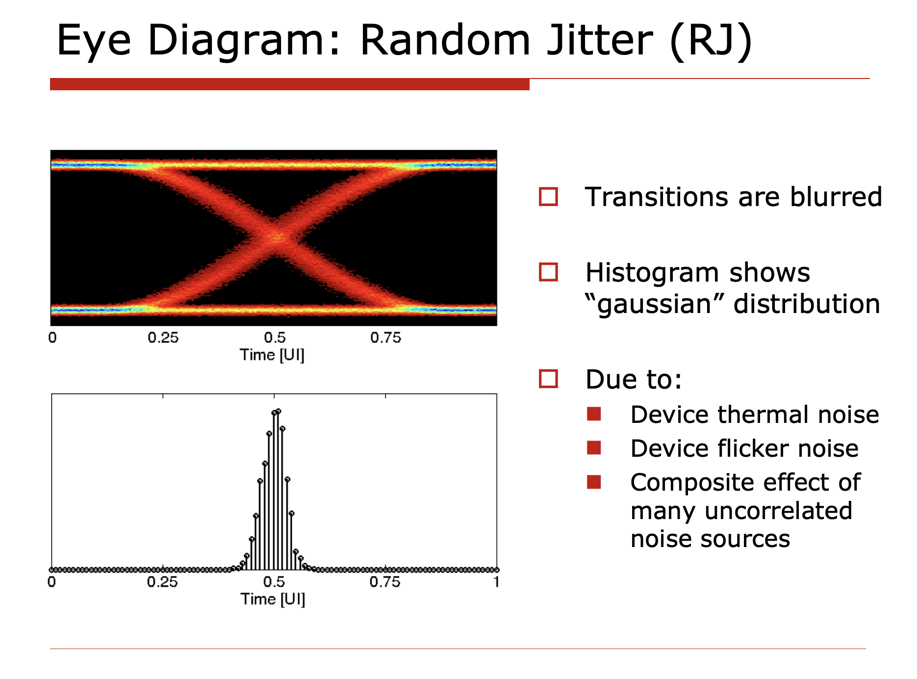
Random jitter is generated from random circuit thermal / flicker noise, which can’t be predicted. The histogram of random jitter is a Gaussian distribution, which is unbounded. Therefore, RMS is a good measure of random jitter.
Period Jitter / Sinusoidal Jitter
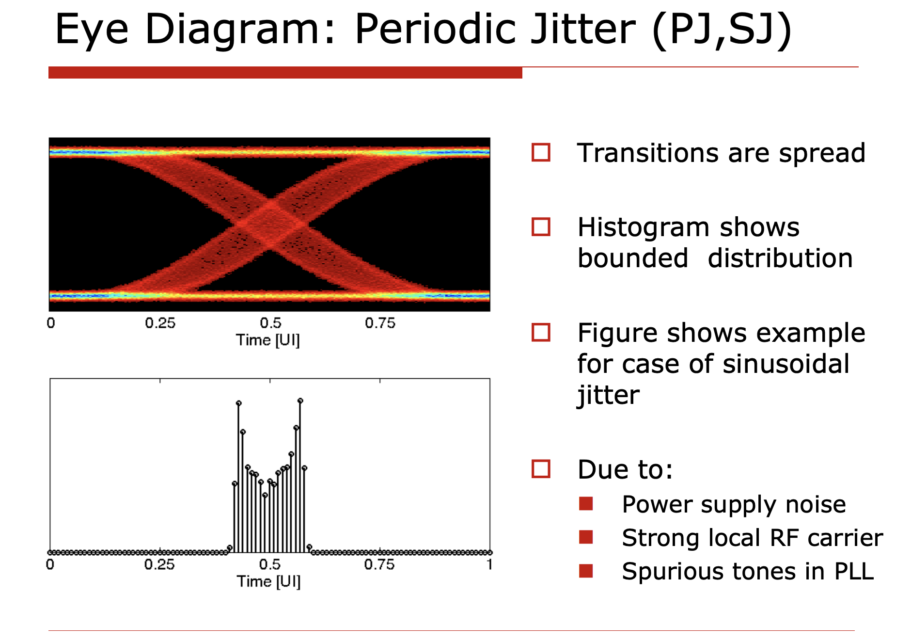
Due to bounded power supply fluctuation, local interference or PLL’s reference clock spur (feedthrough), the output clock has a periodic push-pull behavior. These jitters are usually bounded and have a sinusoidal shape over time.
Data-Dependent Jitter (DDJ), Inter-Symbol Interference (ISI)
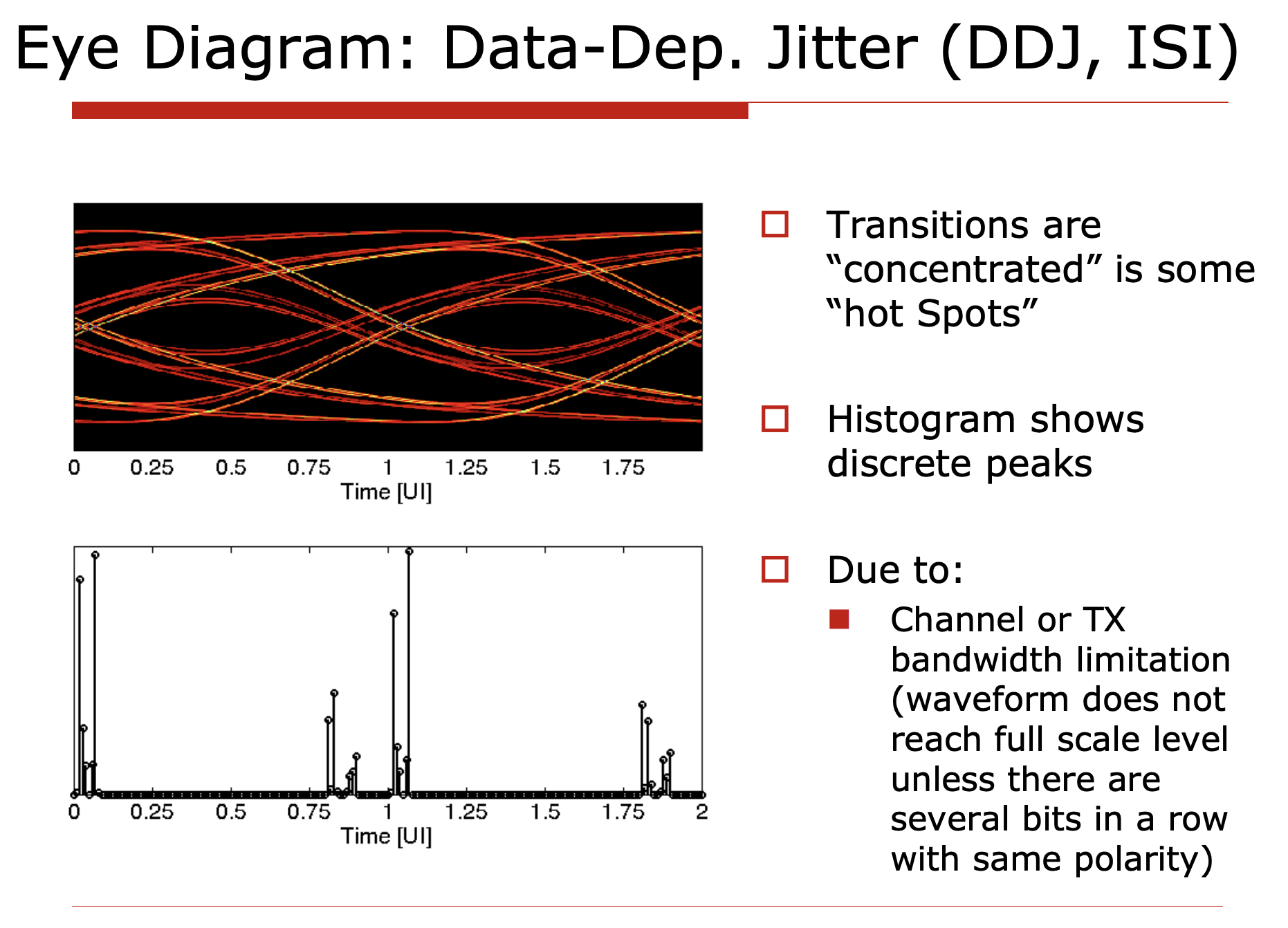
Data-dependent jitter happens when the output data signal is affected by the previous data bits, since the channel has a finite bandwidth. This is also known as inter-symbol interference (ISI). The histogram of DDJ is usually bounded, and the shape of the histogram concentrates around some discrete values.
Duty Cycle Distortion (DCD)
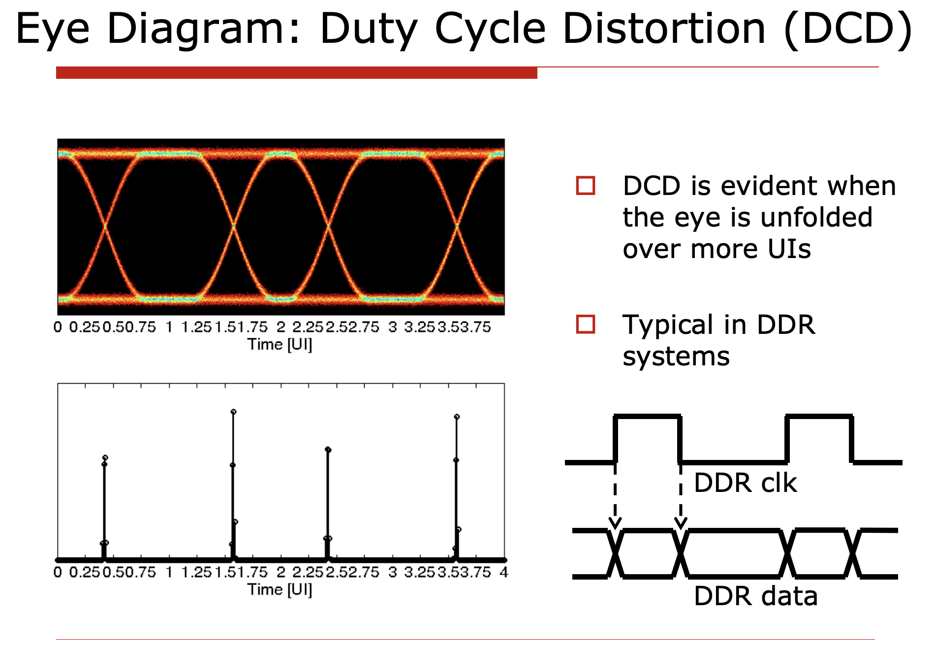
Duty cycle distortion (DCD) is a special case of data-dependent jitter, where the output clock signal has a duty cycle that is not 50%. DCD is a lot more pronounced when the system uses DDR (double data rate) signaling, where the clock signal is used to sample the data signal at both rising and falling edges. To extend the example, if the clock is quarter rate, then the quadrature error of the clock signal will also be a special case of DCD.
Rise/Fall Time Assymmetry
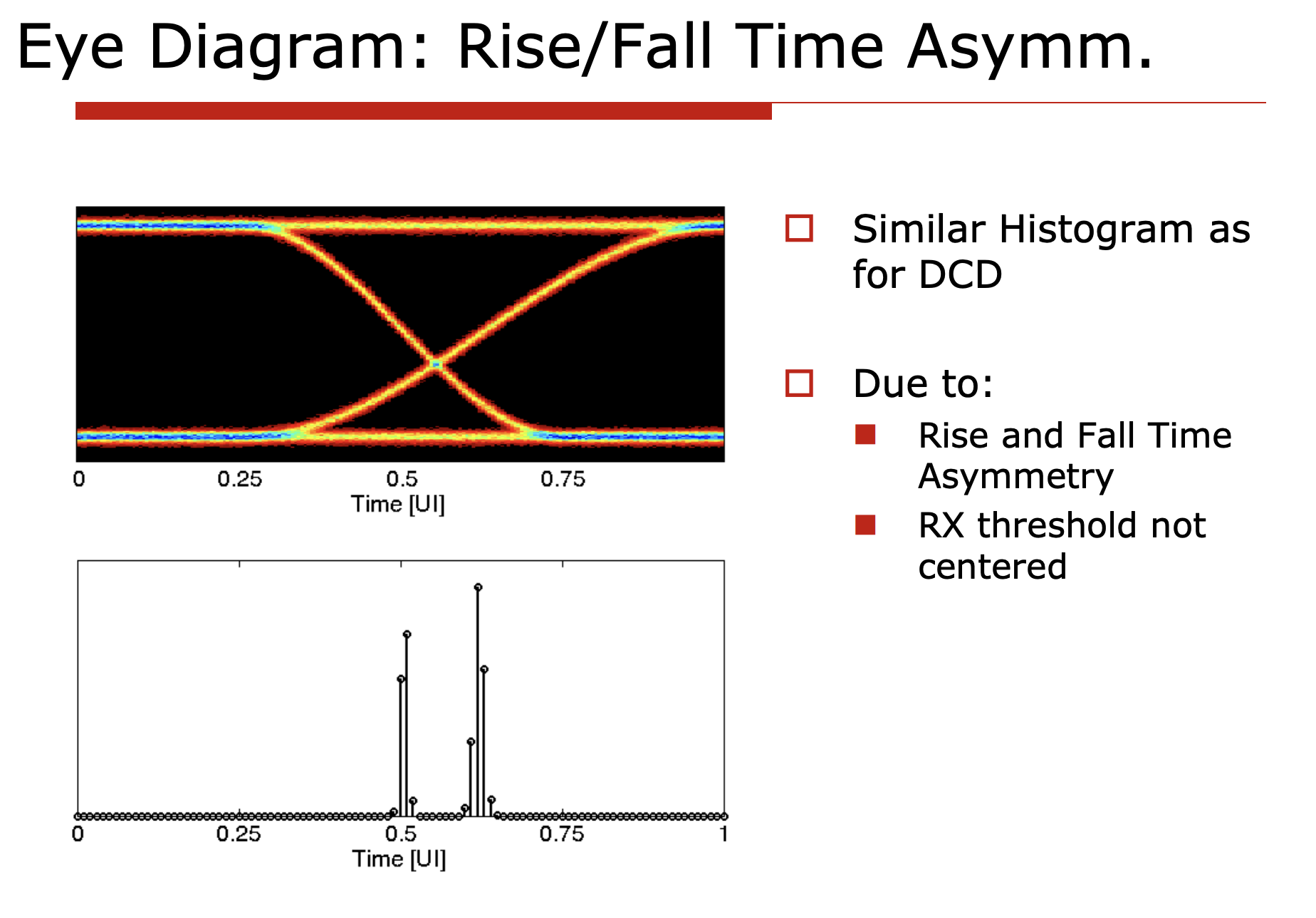
If we didn’t center the RXAFE sampling threshold at the midpoint of the signal coming in, or due to process variation the rise/fall time of the signal is not symmetric, then the clock edges will be shifted to one side.
Putting things together
In real practice it’s impossible to separate all the different types of jitter and they tend to come altogether, like this:
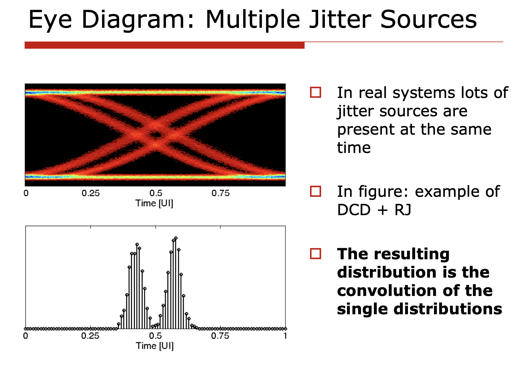
If you have taken basic statistics courses, you will understand that the histogram of different distributions are constructed in such a way that the PDFs are all convolved together, i.e.:
$$ PDF_{total} = PDF_{RJ} \circledast PDF_{PJ} \circledast PDF_{DDJ} \circledast PDF_{DCD} \circledast PDF_{Rise/Fall} \circledast \ldots $$Where $PDF$ is the probability density function of each type of jitter.
Jitter Decomposition
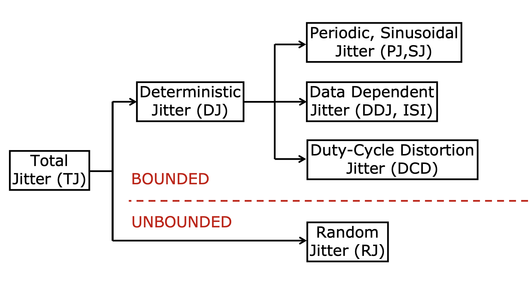
- For any jitter with bounded distribution, we call it Deterministic Jitter (DJ).
- For any jitter with unbounded distribution, we call it Random Jitter (RJ).
- The result of DJ and RJ together is called Total Jitter (TJ).
Gaussian Q Function: from RMS value to histogram
The following facts are worth noting:
- Deterministic jitter comes from a deterministic source. For example if we know the entire circuit behavior and vdd fluctuation profile, we are able to predict all the future jitter samples one by one. However, this is very tedious and impractical, therefore we usually characterize the deterministic jitter by its peak-to-peak value.
- Determinstic jitter compress the available eye width, but it doesn’t affect the bit error rate (BER).
- Suppose we have an ideal eye margin of 100ps, and the deterministic jitter has a peak-to-peak value of 20ps, then the effective eye margin is 80ps. No matter how long we measure the link within the 80ps eye margin, we will never see a bit error.
- Random jitter, on the other hand, is unbounded and can cause bit errors. For a Gaussian process, if we observe it long enough, we will eventually see the process spanning the entire real line $\mathbb{R}$.
Because of 3, in order to characterize a link we’ll need to pre-define a bit error rate (BER) target, and then we can calculate the required eye margin to achieve that BER target.
To do this we need the Gaussian Q function, which is the tail probability of a standard normal random variable $Z \sim \mathcal{N}(0, 1)$:
$$ Q(x) = P(Z > x) = \frac{1}{\sqrt{2\pi}} \int_x^{\infty} e^{-t^2/2} \, dt = \frac{1}{2} \operatorname{erfc}\left(\frac{x}{\sqrt{2}}\right) $$where $Q(x)$ is the probability that a Gaussian sample lands more than $x$ standard deviations above its mean. Now, if the random jitter has an RMS value of $\sigma_{RJ}$, the probability that an edge drifts more than $\Delta$ away from its ideal position (in one direction) is $Q(\Delta / \sigma_{RJ})$.
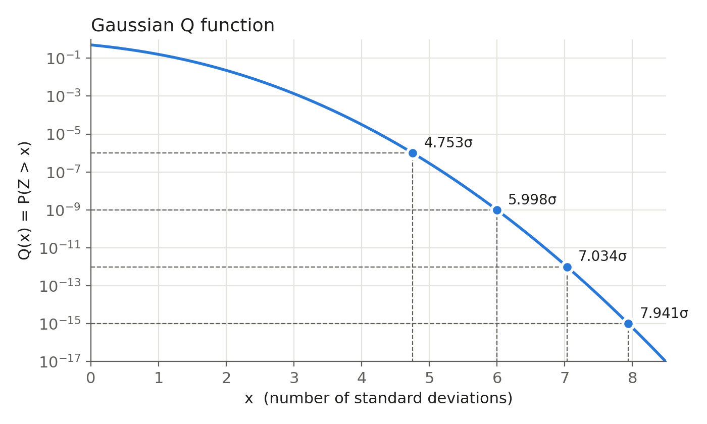
Note that the y-axis is in log scale, and the tail drops by roughly three decades for every extra $\sigma$ in this range.
Let’s look at the eye from the sampler’s point of view. The sampling point sits somewhere between the left edge and the right edge of the eye, and a bit error happens when either edge moves past the sampling point. If we want the error probability to be lower than our BER target, each edge needs to stay at least $Q^{-1}(\text{BER}) \cdot \sigma_{RJ}$ away from the sampling point. Counting both edges, the random jitter takes up:
$$ RJ_{pp}(\text{BER}) = 2 \, Q^{-1}(\text{BER}) \cdot \sigma_{RJ} $$of the eye. Some typical values:
| BER target | $Q^{-1}(\text{BER})$ | $RJ_{pp} / \sigma_{RJ}$ |
|---|---|---|
| $10^{-6}$ | 4.753 | 9.51 |
| $10^{-9}$ | 5.998 | 12.00 |
| $10^{-12}$ | 7.034 | 14.07 |
| $10^{-15}$ | 7.941 | 15.88 |
There are a few things worth noting:
- The Gaussian tail drops very fast.
- Going from $10^{-12}$ to $10^{-15}$, i.e. 1000 times fewer errors, only costs about $1.8\sigma$ of extra eye.
- This is why we can report “TJ at $10^{-12}$” without actually measuring $10^{12}$ bits on the scope. We measure $\sigma_{RJ}$ from a short capture, and extrapolate the tail with $Q^{-1}$.
- The extrapolation is only as good as the Gaussian assumption.
- If the tail is not really Gaussian, for example due to a rare crosstalk event or a supply glitch, the extrapolated number can be way too optimistic.
- Strictly speaking, a bit error can only happen when there is a data transition.
- For random data with transition density $\rho_T \approx 0.5$, some references use $Q^{-1}(\text{BER}/\rho_T)$ instead. The difference is small (7.034 vs 6.937 at $10^{-12}$), and the more conservative form above is the one people usually use.
Putting DJ and RJ together, the total jitter at a given BER is:
$$ TJ(\text{BER}) = DJ_{pp} + 2 \, Q^{-1}(\text{BER}) \cdot \sigma_{RJ} $$and the eye opening left for the receiver is $UI - TJ(\text{BER})$. Suppose we have $DJ_{pp} = 20\text{ps}$ and $\sigma_{RJ} = 1\text{ps}$, then the total jitter at $10^{-12}$ is about $20 + 14.07 = 34.07\text{ps}$.
If we sweep the sampling point across the UI and plot the BER at each position, we get the bathtub curve. The plot below uses a 100ps UI with $DJ_{pp} = 20\text{ps}$, and we can see how the bathtub closes as $\sigma_{RJ}$ increases:
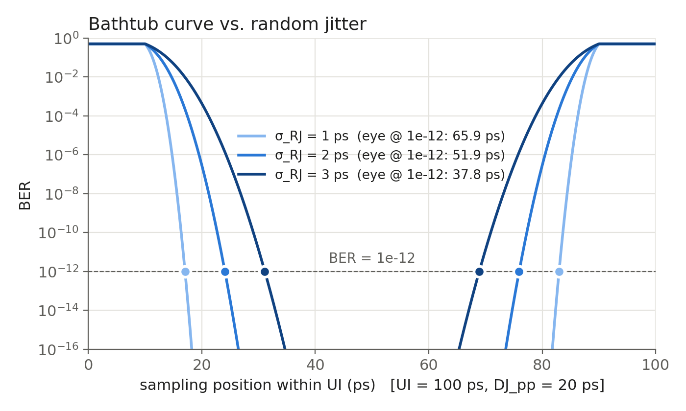
The flat parts near the two edges are the DJ region, where the edge is there for sure and the BER saturates. The slopes are the Gaussian tails of RJ, and the eye width at a given BER is the horizontal distance between the two slopes at that BER level. Going from $\sigma_{RJ} = 1\text{ps}$ to $3\text{ps}$, the eye at $10^{-12}$ shrinks from 65.9ps to 37.8ps, even though DJ doesn’t change at all.
Why Peak-to-Peak Can’t Characterize the Link
Now we can come back to the question at the beginning, and see why a single peak-to-peak number is not enough. Let’s say we have two systems, and we measure 10k hits on each of them:
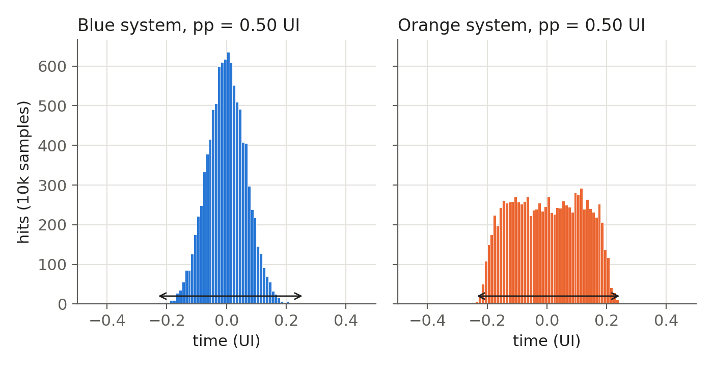
Both histograms have a peak-to-peak value of 0.50 UI. If we only look at peak-to-peak, these are the same link. If we look at the RMS of the whole histogram, the blue system looks a lot better (0.065 UI vs 0.117 UI). However, both conclusions are wrong. The two systems are actually constructed as:
- Blue system: pure random jitter, $\sigma_{RJ} = 0.065\text{UI}$.
- Orange system: deterministic jitter uniformly distributed within $\pm 0.2\text{UI}$, plus random jitter with $\sigma_{RJ} = 0.02\text{UI}$.
Now let’s plot the bathtub curves of both systems, assuming a transition density of 0.5 so that the BER saturates at 0.5 near the edges:
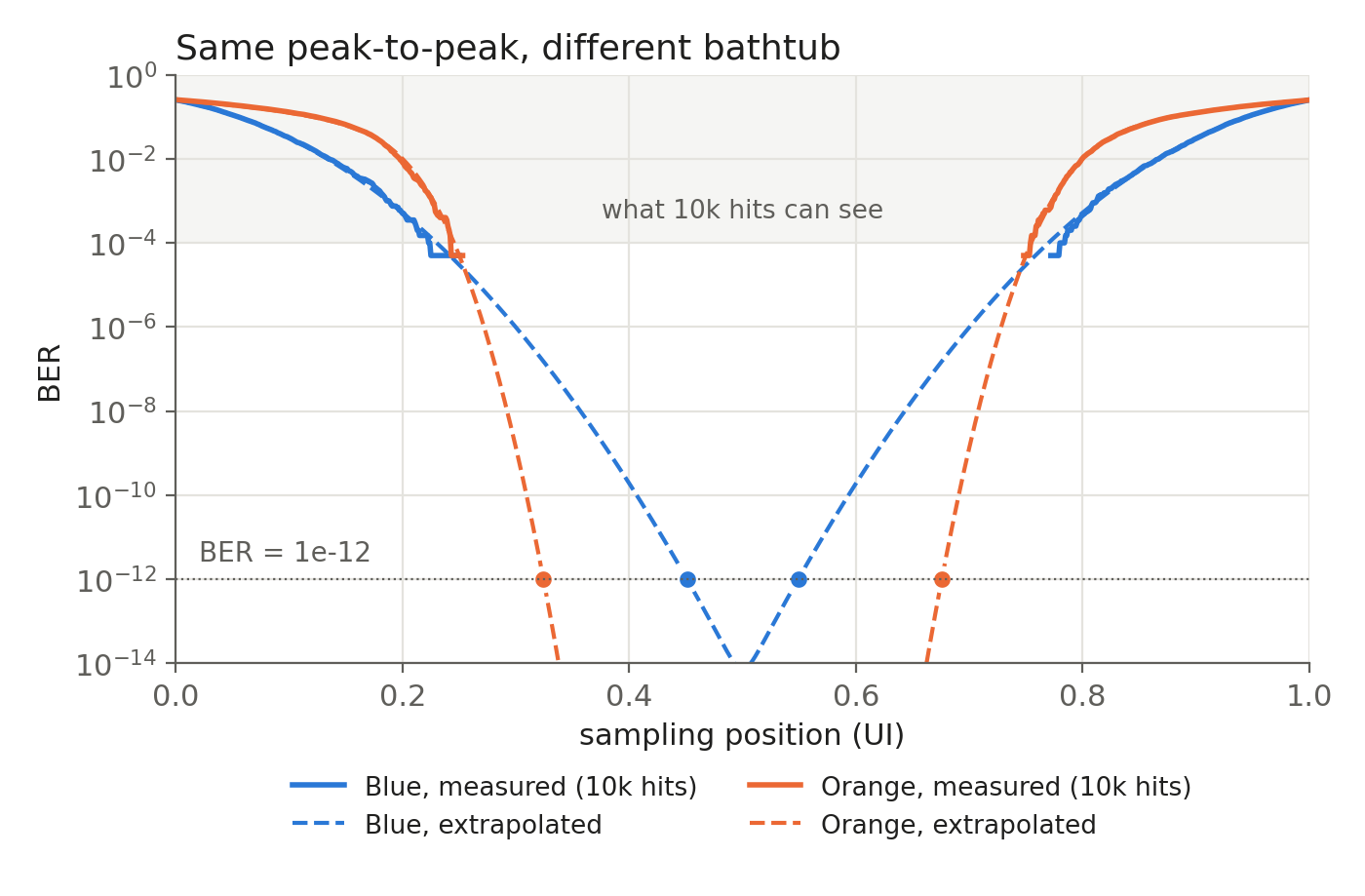
The solid lines are what we can measure from 10k hits, which only reaches down to about $10^{-4}$. Within this region the two bathtubs look similar, and the blue one even looks slightly better. But the orange system has much steeper slopes, since its tail is set by a 0.02UI Gaussian, while the blue tail is set by a 0.065UI Gaussian. Once we extrapolate down to low BER, the two systems are completely different:
| BER | Blue eye opening | Orange eye opening |
|---|---|---|
| $10^{-3}$ | 0.63 UI | 0.55 UI |
| $10^{-6}$ | 0.40 UI | 0.46 UI |
| $10^{-9}$ | 0.24 UI | 0.40 UI |
| $10^{-12}$ | 0.10 UI | 0.35 UI |
At $10^{-12}$ the orange system has about 3.5 times the eye opening of the blue system, even though both of them have the same peak-to-peak value, and the blue one has a smaller RMS value.
The peak-to-peak value also depends on how long we measure. If we keep collecting more samples:
| Number of hits | Blue pp | Orange pp |
|---|---|---|
| $10^3$ | 0.43 UI | 0.47 UI |
| $10^4$ | 0.49 UI | 0.51 UI |
| $10^5$ | 0.57 UI | 0.54 UI |
| $10^6$ | 0.65 UI | 0.56 UI |
| $10^7$ | 0.68 UI | 0.58 UI |
The blue peak-to-peak keeps growing, since a Gaussian is unbounded and we will always see a larger outlier if we wait long enough. The orange peak-to-peak grows much slower, since most of its spread comes from the bounded DJ, and only the small RJ part keeps growing.
There are a few things worth noting:
- Peak-to-peak is only meaningful together with the number of samples, and even then it only tells us about the BER level that the measurement can reach.
- With 10k hits, peak-to-peak roughly tells us the eye at around $10^{-4}$, which says nothing about the eye at $10^{-12}$.
- Peak-to-peak and the RMS of the whole histogram both mix DJ and RJ into a single number.
- What actually determines the eye at low BER is the slope of the bathtub, i.e. $\sigma_{RJ}$, and where the slope starts, i.e. DJ. We need to know both of them separately.
- This is why we need to decompose the jitter into DJ and RJ, which is what the next section does.
End-Tail Fitting
So far we assumed we already know $DJ_{pp}$ and $\sigma_{RJ}$. However, in real practice the scope only gives us one histogram with all the jitter components convolved together, and we need to separate them ourselves. A naive approach is to take the RMS of the whole histogram as $\sigma_{RJ}$, but this is wrong, since the bounded DJ part also contributes to the RMS value even though it never causes a bit error by itself.
The key observation is that far out in the tails, only RJ is left. DJ is bounded, so once we go beyond its worst-case value, the only thing that can push an edge further out is the Gaussian random jitter. Therefore the extreme left of the histogram looks like a Gaussian centered at the left-most DJ position, and the extreme right looks like a Gaussian centered at the right-most DJ position. What happens in the middle doesn’t really matter to us.
This gives us the dual-Dirac model. We pretend all of DJ is just two Dirac delta functions at $\mu_L$ and $\mu_R$, each carrying half of the probability, and convolve them with a Gaussian RJ:
$$ PDF_{model}(t) = \frac{1}{2} \mathcal{N}(t;\, \mu_L, \sigma_L) + \frac{1}{2} \mathcal{N}(t;\, \mu_R, \sigma_R) $$where $\mathcal{N}(t;, \mu, \sigma)$ is the Gaussian PDF with mean $\mu$ and standard deviation $\sigma$. Obviously this model is wrong in the middle of the histogram, but we only need it to be right in the tails, because the tails are what determine the BER.
The procedure goes like this:
- Collect enough samples to see the tails clearly, usually $10^5$ to $10^7$ edges.
- Pick a tail region on each side, where the histogram has clearly left the DJ region but still has enough hits to be statistically meaningful.
- Fit a Gaussian to each tail separately, which gives us $(\mu_L, \sigma_L)$ and $(\mu_R, \sigma_R)$.
- Calculate:
- $DJ_{\delta\delta} = \mu_R - \mu_L$
- $\sigma_{RJ} = (\sigma_L + \sigma_R)/2$
- $TJ(\text{BER}) = DJ_{\delta\delta} + 2 , Q^{-1}(\text{BER}) \cdot \sigma_{RJ}$, same as the formula in the previous section.
Let’s say we have a clock with 20ps peak-to-peak sinusoidal jitter and 2ps RMS random jitter, and we collect 2 million samples. If we plot the histogram on a log scale, the tails look like parabolas (i.e. Gaussian), and the two fitted Gaussians sit right on top of them:
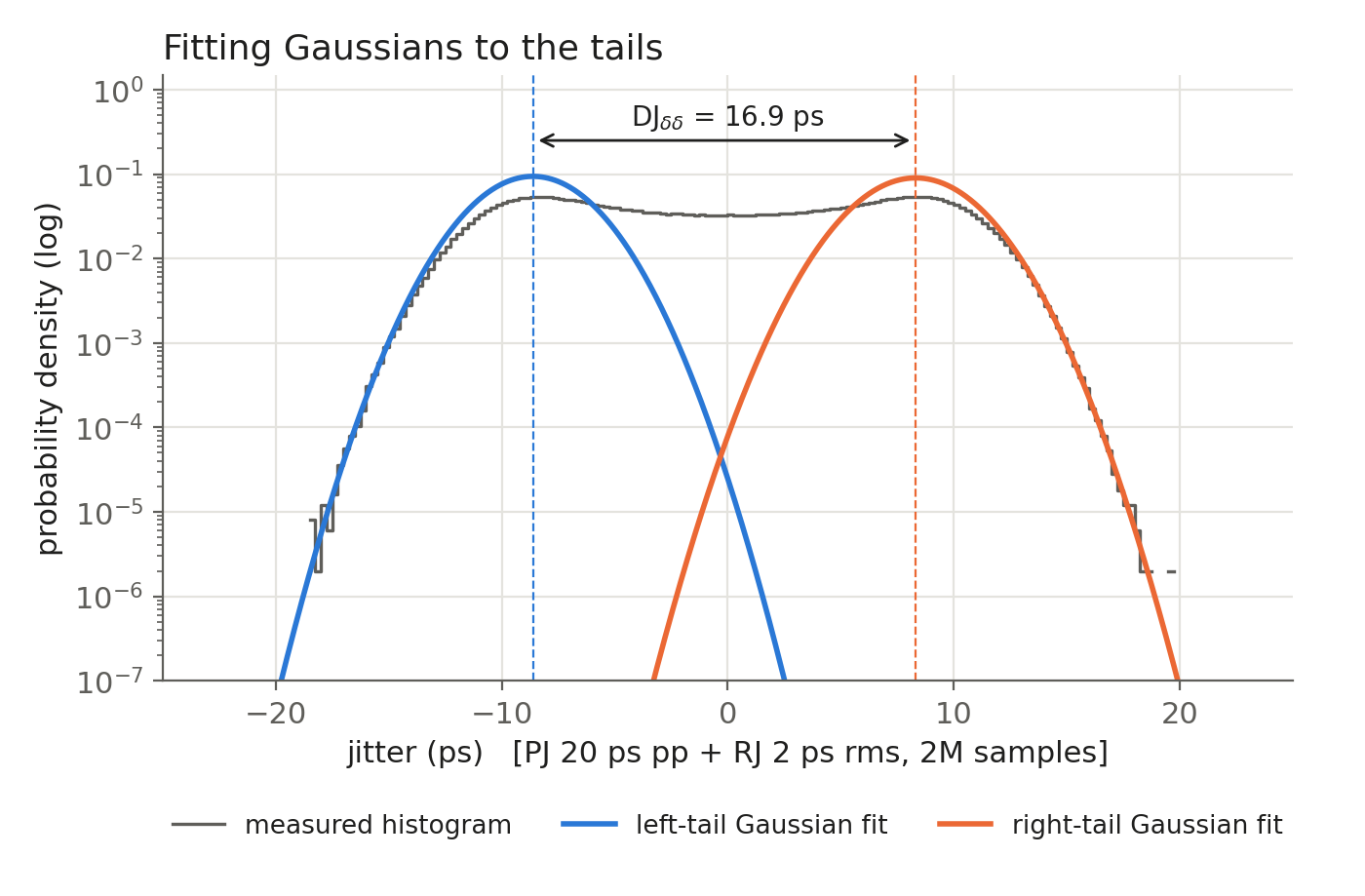
In real practice, fitting a Gaussian directly to the histogram is not easy, since the far tail only has a few hits in each bin. A better way is to use the cumulative probability instead. For a Gaussian tail with weight $1/2$, the probability of landing beyond $t$ on the right side is:
$$ P(X > t) = \frac{1}{2} \, Q\left(\frac{t - \mu_R}{\sigma_R}\right) \quad\Longrightarrow\quad Q^{-1}\big(2 P(X > t)\big) = \frac{t - \mu_R}{\sigma_R} $$which is a straight line in $t$, and the same applies to the left side. So if we plot $Q^{-1}$ of the measured tail probability, also known as the Q-scale, the Gaussian tails become straight lines, and fitting a Gaussian becomes a simple linear regression:
- the slope is $1/\sigma$;
- the zero crossing is $\mu$.
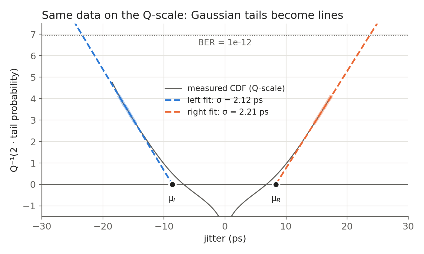
The shaded segments are the region we used for the fit (tail probability between $10^{-5}$ and $10^{-3}$), and the dashed lines are the extrapolation. To get TJ at $10^{-12}$, we extend both lines up to the $Q^{-1}(2 \times 10^{-12})$ level and take the horizontal distance between them. This is pretty much what the scope or BERT software does when it reports “TJ@1e-12” from a measurement much shorter than $10^{12}$ bits.
Comparing the results with the true values:
| Quantity | True value | Tail fit |
|---|---|---|
| RJ (RMS) | 2.00ps | 2.17ps |
| DJ | 20ps (pp) | 16.9ps ($\delta\delta$) |
| TJ @ $10^{-12}$ | 46.6ps | 47.5ps |
| RMS of whole histogram | — | 7.35ps |
There are a few things worth noting:
- $DJ_{\delta\delta}$ is not the same as $DJ_{pp}$.
- A sinusoid spends very little time at its peaks, so the outermost part of the DJ distribution looks like some extra Gaussian spread. The fit takes it as part of $\sigma$, so $DJ_{\delta\delta}$ comes out smaller than 20ps and $\sigma_{RJ}$ comes out slightly larger than 2ps. The two errors cancel each other, and TJ is still within about 2% of the true value. This is actually what the model is designed for: predicting TJ, not recovering the true DJ.
- The fit region matters.
- If we fit too close to the center, DJ leaks in and $\sigma$ is overestimated. If we fit too far out, there are only a few hits and the result is noisy.
- The result is only as good as the Gaussian assumption. A rare non-Gaussian event in the tail, for example crosstalk or a supply glitch, will be extrapolated as if it were RJ.
- Don’t use the RMS of the whole histogram.
- In this example it gives 7.35ps, more than 3 times the real RJ. Plugging it into $2 \times 7.034 \times \sigma$ predicts about 103ps of TJ, more than twice the real value.
- The 47.5ps in the table is calculated from the TJ formula, which uses $Q^{-1}(\text{BER})$. If we read the Q-scale lines exactly at $Q^{-1}(2 \times 10^{-12})$, we get 47.0ps instead. The formula is slightly more conservative, as discussed earlier.