Motivation

Back in the era when Galileo was still alive, he was fascinated by the motion of pendulums. People often say he observed the swinging of a chandelier in the Pisa Cathedral, which led to his groundbreaking studies on the periodicity of pendulums. However, that was pretty much a time when there was no precise measurement of time; how did he know the period of the pendulum accurately? We know later that he used his own pulse as a makeshift timer, which was surprisingly effective for his time – and also surprisingly inaccurate. If his pulse rate varied, the measured period would be correspondingly inaccurate, and leading to significant errors in his observations. You can read more about his experiments with pendulums in this website.

Nonetheless, the period of a pendulum that he established, assuming a small-angle approximation, is remarkably accurate and forms the foundation for understanding the dynamics of pendulums:

where \(T\) is the period of the pendulum, \(L\) is the length of the pendulum, and \(g\) is the acceleration due to gravity. This formula assumes that the amplitude of the pendulum’s swing is small, so that the small-angle approximation holds.

We know later that the pendulum-based timekeeping devices, such as the grandfather clock, relied on this principle. The accuracy of these clocks was limited by the precision of the pendulum’s period, which in turn depended on the length of the pendulum and the local gravitational acceleration. Let’s say we calibrate the clock at a specific time of day, say 12 noon, and we observe the time the second day. Depending on the quality factor (Q factor) of the pendulum, the clock may drift slightly, leading to a discrepancy between the observed time and the actual time.

The Q factor of a pendulum is given by:

where “Energy Stored” refers to the maximum potential energy of the pendulum, and “Energy Lost per Cycle” accounts for the energy dissipated due to air resistance and friction at the pivot point. A higher Q factor indicates a pendulum that loses less energy per cycle, resulting in more accurate timekeeping.

We know later that people managed to inventories of more precise timekeeping devices, such as the quartz crystal oscillator, which significantly improved the accuracy of clocks and watches. The quartz crystal oscillator operates based on the piezoelectric effect, where a quartz crystal vibrates at a very stable frequency when an electric voltage is applied. This frequency can be used to drive a clock mechanism with much higher precision than pendulum-based clocks. However, quartz crystal oscillators are still subject to environmental factors such as temperature changes, which can slightly alter their frequency and, consequently, the accuracy of the timekeeping. The inaccuracy of different kinds of clocks is generalized as the concept of jitter, and we will study how jitter is generated, transfered and tolerated in a modern serial link application through this series of blogs.

Definitions of Different Jitters

This part reflects what Dr. Nicola Da Dalt had in his ISSCC tutorial and Prof. Ali Sheikhoslami had in his ESSERC tutorial. They co-authored a book, Understanding Jitter and Phase Noise: A Circuits and Systems Perspective. We are just giving some convenient definitions from this book.

Absolute Jitter

Suppose we have a periodic signal:

We call $\phi(t)$ the absolute phase deviation of the signal, sometimes also noted as excess phase. If $\phi(t) = 0$, the signal is a perfect sine wave with frequency $f$, and the x-axis crossover time will be such that:

Now, with $\phi(t) \neq 0$, the x-axis crossover time will be shifted by $\phi(t)$, and we can see the actual crossover time as:

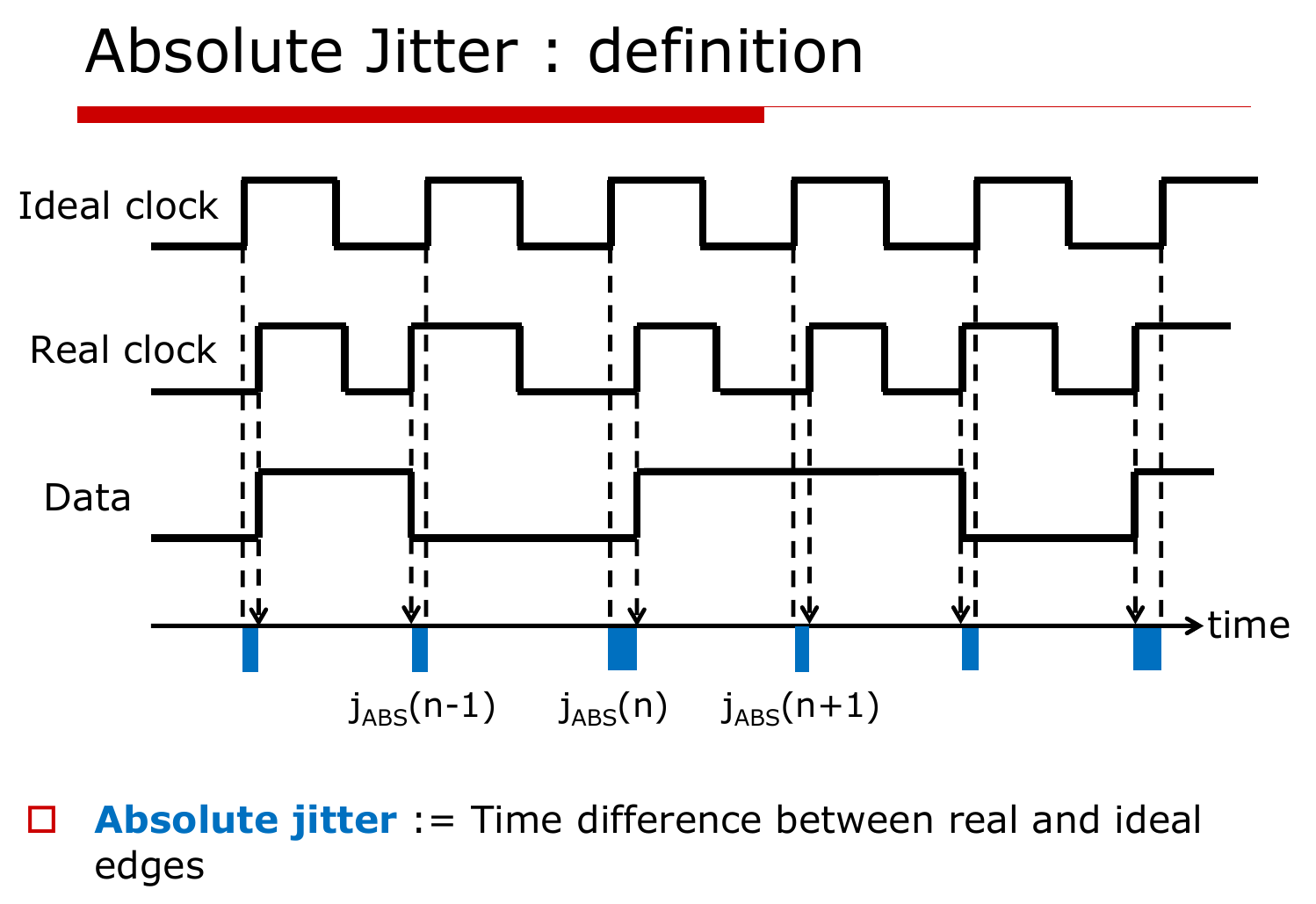
By taking the difference between the actual and ideal crossover times, we can define the absolute jitter as the sequence of time deviations: $j_{ABS}[k]$.

Absolute jitter is a stochastic process, and we can visualize it in time domain using histograms. For a stationary stochastic process, the standard deviation of the absolute jitter doesn’t change with time, which gives us the priviledge to define the RMS absolute jitter as:

⚠️ Warning

This only applies to stationary stochastic jitter process. For a non-stationary process, for example the jitter of a free-running oscillator, the RMS absolute jitter changes with time and longer measurement doesn’t necessarily give a better estimate of the RMS absolute jitter.

Converting Absolute Jitter to Phase Noise

We’ve talked a lot about phase noise in all previous blogs, and we briefly summarize the relationship between absolute jitter and phase noise here.

We know the absolute jitter and excess phase are related by:

Now, if we take PSD on both sides, we have:

where $S_{j_{ABS}}(f)$ is the PSD of absolute jitter, and $S_{\phi}(f)$ is the PSD of excess phase, also known as the phase noise.

Now, Wiener Khinchin theorem tells us how to compute the rms value of absolute jitter, if it’s well defined:

In real practice:

1. We define the upper limit to be the Nyquist frequency of the carrier, otherwise we will double count the jitter from its harmonics.
2. We define the lower limit to be how long we observe the system, usually in terms of kHz. Two reasons here:
   • Most low-frequency jitter can usually be tracked by the system, for example a CDR.
   • It takes very long for low frequency jitter to show up, before which the system might already have done its job.

Relative Jitter

Relative jitter is defined as the difference between one clock edge and another.

We will see later that relative jitter is more useful than absolute jitter in many clock-forwarded applications where we enjoy the benefit of jitter tracking.

N-Cycle Jitter

N-cycle jitter (also called N-period jitter) is the deviation of the time spanned by $N$ consecutive periods from its ideal value $NT$, where $T = 1/f$. Since the ideal edges are exactly $NT$ apart, it is simply the difference of two absolute jitter samples $N$ cycles apart:

Note that this is a special case of relative jitter, where clock 2 is just clock 1 delayed by $N$ cycles. In other words, N-cycle jitter tells us how much a clock disagrees with itself $N$ cycles later.

If the absolute jitter is stationary, the variance of N-cycle jitter can be written in terms of the autocorrelation of absolute jitter:

Two observations:

1. When $N$ is small, the two edges are strongly correlated, $R_{j_{ABS}}(NT) \approx \sigma_{ABS}^2$, and $\sigma_N$ is small. The slow wander is common to both edges and cancels.
2. When $N$ is large enough that the two edges become uncorrelated, $\sigma_N^2 \to 2\sigma_{ABS}^2$.

In the frequency domain, taking the difference $j_{ABS}[k+N] - j_{ABS}[k]$ is a filter with transfer function $1 - e^{-j2\pi f NT}$, whose magnitude squared is $4\sin^2(\pi f N T)$. Therefore:

The $\sin^2$ term is a high-pass filter with a corner around $f \approx 1/(2\pi NT)$: phase noise far below that frequency is suppressed. This is why N-cycle jitter is well defined even for a free-running oscillator, where $\sigma_{ABS}$ is not. For a free-running oscillator dominated by white frequency noise ($S_{\phi} \propto 1/f^2$), the variance grows linearly with $N$, i.e. $\sigma_N \propto \sqrt{N}$, the familiar random-walk behavior of jitter accumulation.

The divided clock of a PLL is a good example of N-cycle jitter: the PLL tracks the input clock, so the divided clock is correlated with itself over many cycles. The N-cycle jitter of the divided clock is much smaller than its absolute jitter, and it is what matters for timing closure in synchronous digital logic.

Period Jitter

Period jitter is the N-cycle jitter with $N = 1$, i.e. the deviation of each individual period from the ideal period:

where $T[k] = \text{cross,actual}[k+1] - \text{cross,actual}[k]$ is the $k$-th actual period. Plugging $N = 1$ into the result above:

Period jitter is what matters for timing closure in synchronous digital logic: if a period is shorter than nominal, the setup margin of every flip-flop clocked by it shrinks by the same amount.

Cycle-to-Cycle Jitter

Cycle-to-cycle jitter is the difference between two adjacent periods:

So period jitter is the first difference of absolute jitter, and cycle-to-cycle jitter is the second difference. Each difference applies another $|1 - e^{-j2\pi fT}|^2 = 4\sin^2(\pi f T)$ to the PSD:

Cycle-to-cycle jitter rejects low-frequency phase noise even more strongly than period jitter, so it mostly captures sudden period changes, such as those caused by supply glitches or a divider/PLL hopping between states. If the period jitter samples are uncorrelated, $\sigma_{CC} = \sqrt{2},\sigma_P$.