Control engineers like to come up with novel control algorithms to either reduce the impact of disturbances on the system or improve the overall performance of the control system; however, there is always one assumption that they like to make: the system is fully observable and the state of the system can be accurately measured. When I was taking EE222: Nonlinear Systems at UC Berkeley, I asked whether all system states are observable, and the professor said “yes” during the first lecture. He explained this is not true in general, and suggested that I take another course on state estimation. Unfortunately, I didn’t end up taking that class since I had already completed my course requirements for my PhD study.
However, the ability to always correctly measure the state of the system is not guaranteed in practice. I design PLLs, which are typical closed-loop control systems, but there are factors that make the phase measurement less accurate. Latency in measurement, quantization noise in the TDC, and other environmental disturbances all contribute to the inaccuracy of the state measurement.
Rudolf Kalman did a thorough analysis of the problem of state estimation in the presence of noise and uncertainty, and one of the most significant contributions he made was the development of the Kalman filter, which provides an optimal recursive solution for estimating the state of a dynamic system from noisy measurements. I’m going to use this post to explain the intuition behind the Kalman filter and how it works in practice. The illustrative example is from this website.
The Noiseless Dynamic Model
Let’s say we are designing a radar system that tracks the position of an aircraft. Let’s say the aircraft moves in a straight line at a constant velocity. At the initial time $t_0$, we measure the position of the aircraft to be $r_{t_0}$, and the velocity to be $v_0$. By elementary physics we know the future position of the aircraft at time $t$ can be predicted as:
$$ r_t = r_{t_0} + v_0 (t - t_0) $$If there is neither measurement noise nor system disturbance, by measuring the initial condition once, we are able to accurately predict the future state of the system at any time $t$, without even looking at the measurements again. Indeed, for any noiseless system, the states at any future time are purely deterministic and can be computed directly from the initial conditions. Any closed-loop control policy will be identical to any open-loop control policy because we don’t need any feedback from the measurements.
Here, the equation above is usually known as the dynamic model or state transition model, which describes how the state of the system evolves over time. In reality, there are two factors affecting the evolution of the states:
- System disturbance: The actual system may be influenced by external disturbances that are not accounted for in the dynamic model.
- This can be, for example, the wind affecting the aircraft’s motion, or disturbance in the thrust of the aircraft.
- Measurement noise: The measurements of the state are often corrupted by noise, making it difficult to accurately determine the true state of the system.
- This can be the sensor inaccuracies, quantization noise, etc.
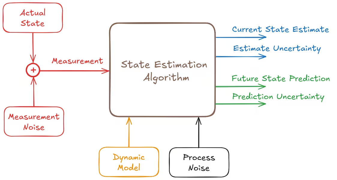
Our goal is to get the best estimate of the true state of the system in the future, by combining our modeling of the system dynamics with the noisy measurements.
Initialization
Starting from $t_0$, let’s define the state vector at time $t$ as:
$$ \bm{x} = \begin{pmatrix} r \\ v \end{pmatrix} $$where $r$ is the position and $v$ is the velocity. $\bm{x}$ is the true state vector.
On the other hand, if we were to measure the system, we denote our measurement using the letter $z$. Suppose at the initial time, our measurement is such that
$$ \bm{z}_0 = \begin{pmatrix} 10000 \\ 200 \end{pmatrix} $$To perform initialization, we make it so that the estimated true state vector at the initial time is equal to the measurement:
$$ \hat{\bm{x}}_{0,0} = \bm{z}_0 = \begin{pmatrix} 10000 \\ 200 \end{pmatrix} $$Notice that we are using $\hat{\bm{x}}_{0,0}$ to denote the estimated true state vector at the initial time.
Measurement Noise
We characterize the degree to which we can trust the measurement by the measurement covariance matrix $\bm{R}$. Let’s say in this example,
$$ \bm{R} = \begin{pmatrix} \sigma_r^2 & \sigma_{rv} \\ \sigma_{rv} & \sigma_v^2 \end{pmatrix} = \begin{pmatrix} 16 & 0 \\ 0 & 0.25 \end{pmatrix} $$For simplicity, we assume that the measurements for position and velocity are fully uncorrelated, hence the covariance matrix is diagonal.
Prediction
We now predict the next state. Assume our measurement equipment measures every 5 s, therefore $\Delta t = 5$ s and $t_1 = 5$ s.
Our next state $\bm{x}_1$ will be such that
$$ \bm{x}_1 = \begin{pmatrix} r_1 \\ v_1 \end{pmatrix} = \begin{pmatrix} r_0 + v_0 \Delta t \\ v_0 \end{pmatrix} = \begin{pmatrix} 1 & \Delta t \\ 0 & 1 \end{pmatrix} \begin{pmatrix} r_0 \\ v_0 \end{pmatrix} = \bm{F} \bm{x}_0 $$Here we call $\bm{F}$ the state transition matrix.
Therefore, one possible prediction, from our $\hat{\bm{x}}_{0,0}$, is
$$ \hat{\bm{x}}_{1,0} = \bm{F} \hat{\bm{x}}_{0,0} \tag{*} $$
We call equation (*) the prediction equation or state extrapolation equation.
Here $\hat{\bm{x}}_{1,0}$ is the estimated state at time $t_1$, predicted at $t_0$. Equation (*) shows the prediction step in the Kalman filter. To generalize to any time step $n$, we have
$$ \hat{\bm{x}}_{n+1, n} = \bm{F} \hat{\bm{x}}_{n, n} + \bm{G} \bm{u}_n $$where $\bm{G}$ is the control input transition matrix and \( \bm{u}_n \) is the control input at time step $n$. If there is no control policy, then our system is uncontrolled and the term \( \bm{G} \bm{u}_n \) can be omitted.
Covariance Matrix Extrapolation
At the next time step, our covariance matrix will not stay where it was, because erroneous measurement will lead to an increase in uncertainty.
The covariance extrapolation is given by:
$$ \bm{P}_{n+1, n} = \bm{F} \bm{P}_{n, n} \bm{F}^\top + \bm{Q} $$where \( \bm{P}_{n+1, n} \) is the predicted covariance matrix at time step $n+1$, \( \bm{P}_{n, n} \) is the updated covariance matrix at time step $n$, and $\bm{Q}$ is the process noise covariance matrix.
Let’s assume that, due to the wind, the standard deviation of the random acceleration is \( \sigma_a = 0.2\ \text{m/s}^2 \). Therefore, the process noise covariance matrix is
$$ \bm{Q} = \begin{pmatrix} \Delta t^4 / 4 & \Delta t^3 / 2 \\ \Delta t^3 / 2 & \Delta t^2 \end{pmatrix} \sigma_a^2 = \begin{pmatrix} 156.25 & 62.5 \\ 62.5 & 25 \end{pmatrix} \times 0.04 = \begin{pmatrix} 6.25 & 2.5 \\ 2.5 & 1 \end{pmatrix} $$Since we initialized the state with the first measurement, we also inherit its uncertainty as the initial covariance, \( \bm{P}_{0,0} = \bm{R} \). Therefore, at the next time step, the squared uncertainty of our prediction is
$$ \bm{P}_{1, 0} = \bm{F} \bm{P}_{0, 0} \bm{F}^\top + \bm{Q} = \begin{pmatrix} 28.5 & 3.75 \\ 3.75 & 1.25 \end{pmatrix} $$Iteration
Now we’ve done the prediction step. Let’s say after 5 seconds, we manage to perform a new measurement:
$$ \bm{z}_1 = \begin{pmatrix} 11020 \\ 202 \end{pmatrix} $$Let’s say now at $t_1$, the measurement covariance matrix is
$$ \bm{R}_1 = \begin{pmatrix} 36 & 0 \\ 0 & 2.5 \end{pmatrix} $$Now it’s time to pause and look at what we have. We have the predicted state \( \hat{\bm{x}}_{1,0} \), and the measured state \( \bm{z}_1 \). Which one shall we pick?
Intuitively, trusting the measurement will be preferable since it provides the most current information about the system’s state. However, if we compare the prediction covariance \( \bm{P}_{1,0} \) with the measurement covariance \( \bm{R}_1 \):
$$ \bm{P}_{1,0} = \begin{pmatrix} \textcolor{#eb6834}{28.5} & 3.75 \\ 3.75 & \textcolor{#eb6834}{1.25} \end{pmatrix}, \quad \bm{R}_1 = \begin{pmatrix} \textcolor{#2a78d6}{36} & 0 \\ 0 & \textcolor{#2a78d6}{2.5} \end{pmatrix} $$We spot something interesting. The measurement actually shows higher uncertainty for both the position and velocity components compared to our prediction, which means that our prediction is more reliable at this point.
Which one shall we pick, the prediction or measurement? Rudolf Kalman says “let’s do both” and came up with this equation:
$$ \hat{\bm{x}}_{1,1} = \bm{K}_1 \bm{z}_1 + (\bm{I} - \bm{K}_1) \hat{\bm{x}}_{1,0} = \underbrace{\hat{\bm{x}}_{1,0}}_{\text{prediction}} + \underbrace{\bm{K}_1 (\bm{z}_1 - \hat{\bm{x}}_{1,0})}_{\text{correction}} $$Here we call \( \bm{K}_1 \) the Kalman gain, which determines how much we should trust the measurement compared to the prediction. We also call \( \bm{z}_1 - \hat{\bm{x}}_{1,0} \) the innovation or measurement residual, which represents the difference between the actual measurement and the predicted state.
In real applications, the states are not always immediately observable. The measurement is usually a transformed result of the states:
$$ \bm{z}_n = \bm{H} \bm{x}_n $$In our example, the output matrix $\bm{H}$ is the identity matrix since we can directly observe both the position and velocity.
Finding the Kalman Gain
The optimal Kalman gain makes it such that the posterior covariance matrix is minimized. Mathematically, it is given by:
$$ \bm{K}_n = \bm{P}_{n, n-1} \bm{H}^\top (\bm{H} \bm{P}_{n, n-1} \bm{H}^\top + \bm{R}_n)^{-1} $$For our example, we can calculate the first Kalman gain as:
$$ \begin{align*} \bm{K}_1 &= \bm{P}_{1,0} \bm{H}^\top (\bm{H} \bm{P}_{1,0} \bm{H}^\top + \bm{R}_1)^{-1} \\ &= \begin{pmatrix} 0.4074 & 0.5926 \\ 0.0412 & 0.2922 \end{pmatrix} \end{align*} $$Substituting the Kalman gain into the update equation, we get the posterior state estimate:
$$ \begin{align*} \hat{\bm{x}}_{1,1} &= \hat{\bm{x}}_{1,0} + \bm{K}_1 (\bm{z}_1 - \hat{\bm{x}}_{1,0}) \\ &= \begin{pmatrix} 11009.33 \\ 201.41 \end{pmatrix} \end{align*} $$Quantify the Posterior Covariance
Aside from just estimating the posterior state, it is also important to quantify the uncertainty of this estimate. This is done through the posterior covariance matrix, which is given by the Joseph form:
$$ \bm{P}_{n,n} = (\bm{I} - \bm{K}_n \bm{H}) \bm{P}_{n,n-1} (\bm{I} - \bm{K}_n \bm{H})^\top + \bm{K}_n \bm{R}_n \bm{K}_n^\top $$We can also use the simplified posterior covariance update:
$$ \bm{P}_{n,n} = (\bm{I} - \bm{K}_n \bm{H}) \bm{P}_{n,n-1} $$WarningThe simplified posterior covariance update is only valid when the Kalman gain is optimal. In practice, using the Joseph form ensures numerical stability and accuracy.
Now, if we use the simplified posterior covariance update, we get:
$$ \bm{P}_{1,1} = (\bm{I} - \bm{K}_1 \bm{H}) \bm{P}_{1,0} = \begin{pmatrix} 14.67 & 1.48 \\ 1.48 & 0.73 \end{pmatrix} $$Let’s do a comparison among the three covariance matrices: the prior covariance \( \bm{P}_{1,0} \), the posterior covariance \( \bm{P}_{1,1} \) and the measurement covariance \( \bm{R}_1 \).
$$ \bm{P}_{1,1} = \begin{pmatrix} \textcolor{#1baf7a}{14.67} & 1.48 \\ 1.48 & \textcolor{#1baf7a}{0.73} \end{pmatrix}, \quad \bm{P}_{1,0} = \begin{pmatrix} \textcolor{#eb6834}{28.5} & 3.75 \\ 3.75 & \textcolor{#eb6834}{1.25} \end{pmatrix}, \quad \bm{R}_1 = \begin{pmatrix} \textcolor{#2a78d6}{36} & 0 \\ 0 & \textcolor{#2a78d6}{2.5} \end{pmatrix} $$We can see that after the Kalman update, the posterior covariance has its diagonal elements reduced compared to the prior covariance, indicating an increased confidence in the state estimates.
Pseudo Code
Putting everything together, the Kalman filter is just two steps repeated for every new measurement: predict, then update.
 1initialize:  x = z_0,  P = R_0
 2
 3for each new measurement z_n with covariance R_n:
 4    # predict
 5    x = F x                                    # state extrapolation
 6    P = F P F^T + Q                            # covariance extrapolation
 7
 8    # update
 9    K = P H^T (H P H^T + R_n)^(-1)             # Kalman gain
10    x = x + K (z_n - H x)                      # state update
11    P = (I - K H) P (I - K H)^T + K R_n K^T    # covariance update (Joseph form)
Example: Inverted Pendulum on a Cart
Let’s close with the most famous toy problem in control: balancing an inverted pendulum on a cart, and bringing the cart back home. I’ll reuse the setup from my EE222 homework, and ask a simple question: given the same controller, how much does the state estimate we feed into it matter?
The System
Linearized around the upright position, the pendulum angle $\theta$ and the cart position $s$ follow:
$$ \begin{align*} (J + mL^2)\ddot{\theta} - mgL\theta &= mL\ddot{s} \\ (M + m)\ddot{s} + b\dot{s} - mL\ddot{\theta} &= F \end{align*} $$where $F$ is the force applied to the cart, and $\theta$ is measured from the upright position, positive when the pendulum leans toward $-s$ (pushing the cart toward $+s$ makes the pendulum lean back, i.e. increases $\theta$). I use $M = 25$ kg, $m = 20$ kg, $L = 9.81$ m, $J = mL^2/3$ and no friction ($b = 0$). With the state vector \( \bm{x} = (\theta, s, \dot{\theta}, \dot{s})^\top \), this gives
$$ \bm{A} = \begin{pmatrix} 0 & 0 & 1 & 0 \\ 0 & 0 & 0 & 1 \\ 1.125 & 0 & 0 & 0 \\ 4.905 & 0 & 0 & 0 \end{pmatrix}, \quad \bm{B} = \begin{pmatrix} 0 \\ 0 \\ 0.00255 \\ 0.0333 \end{pmatrix} $$The open-loop system has a pole at $+1.06$ rad/s: left alone, any tilt grows by about $e$ every second.
The “true” pendulum in the simulation is the full nonlinear model, integrated with RK4. The Kalman filter only knows the linearized model above, discretized at 100 Hz, so there is some model mismatch on top of the noise.
The Controller
To bring the cart back to the origin, I use the large-area-of-attraction controller from a later homework, which divides the pendulum feedback by $\cos\theta$ to cancel the nonlinearity, and saturates the cart feedback so that a large cart offset doesn’t produce a huge force:
$$ F = \frac{-k_\theta \theta - k_{\dot{\theta}} \dot{\theta}}{\cos\theta} - \frac{k_s s}{1 + K_1 |s|} - \frac{k_{\dot{s}} \dot{s}}{1 + K_2 |\dot{s}|} $$The gains come from an LQR design with \( \bm{Q}_{LQR} = \text{diag}(10^4, 100, 100, 100) \) and $R_{LQR} = 0.1$, which gives
$$ (k_\theta, k_s, k_{\dot{\theta}}, k_{\dot{s}}) = (2903, -31.6, 3157, -129.9) $$with closed-loop poles at $-1.24 \pm 0.38j$ and $-0.62 \pm 0.29j$, and I use $K_1 = K_2 = 0.05$. Unlike the homework, I also limit the force to $\pm 1$ kN, because a real motor can’t push infinitely hard.
The Noise
- Process noise: random gusts push the cart with a force of standard deviation 20 N, held constant over each 10 ms step. Since the gust enters exactly like $F$ does, the process noise covariance is \( \bm{Q} = \bm{G}\bm{G}^\top \sigma_w^2 \), where $\bm{G}$ is the discretized input matrix, the same construction as the random acceleration in our radar example.
- Measurement noise: we only have sensors for the angle and the cart position, with standard deviations of 0.002 rad (about 0.11°, a decent encoder) and 1 cm. The velocities $\dot{\theta}$ and $\dot{s}$ are not measured, so
Three Ways to Get the State
All three runs start with the pendulum at $\theta = 0.3$ rad (17°) and the cart 2 m away from home, see exactly the same gusts and the same sensor noise, and use exactly the same controller. The only difference is the state estimate \( \hat{\bm{x}} \) that the controller sees:
- Prediction only: run the model, \( \hat{\bm{x}}_{n+1} = \bm{F}\hat{\bm{x}}_n + \bm{G}u_n \), and never look at the sensors.
- Measurement only: trust the sensors completely, and get the velocities by finite differences, e.g. \( \hat{\dot{\theta}}_n = (z_{\theta,n} - z_{\theta,n-1}) / \Delta t \).
- Kalman filter: predict with the model, then correct with the measurement, exactly like the pseudo code above.
Here are the three runs side by side, animated in real time on a shared clock. The gray arrow on each cart shows the control force.
On the right of each run is the Lyapunov function that comes with the LQR design, evaluated on the true state:
$$ V(\bm{x}) = \bm{x}^\top \bm{P} \bm{x} $$where $\bm{P}$ is the solution of the Riccati equation that we solved to get the LQR gains in the first place. For the linearized closed loop, it decreases along every trajectory, \( \dot{V} = -\bm{x}^\top (\bm{Q}_{LQR} + \bm{K}^\top R_{LQR} \bm{K}) \bm{x} < 0 \), so a healthy run should show $V$ sliding steadily downhill.
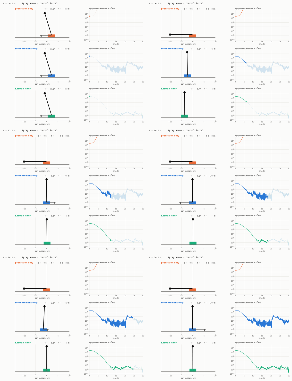
The Kalman run does exactly that: $V$ decays by about four orders of magnitude, and then settles at a small floor where the random gusts keep kicking the state a little. The measurement-only run starts out the same way, but once the noise takes over, $V$ keeps bouncing between roughly 10 and 1000: the controller is constantly undoing the damage its own noisy velocity estimate causes. And for prediction only, $V$ shoots off the top of the plot as the pendulum falls.
The results:
| Prediction only | Measurement only | Kalman filter | |
|---|---|---|---|
| Pendulum | Falls at $t = 5.2$ s | Balanced, but wobbly | Balanced |
| RMS angle once settled (last 10 s) | — | 1.39° | 0.11° |
| Final cart offset (from 2 m) | — | 11 cm | 1 cm |
| RMS error of \( \hat{\theta} \) | 30° | 0.11° | 0.021° |
| RMS error of \( \hat{\dot{\theta}} \) | 26°/s | 16°/s | 0.21°/s |
| RMS control force | 147 N | 699 N | 64 N |
| Time at the force limit | 0% | 28% | 0% |
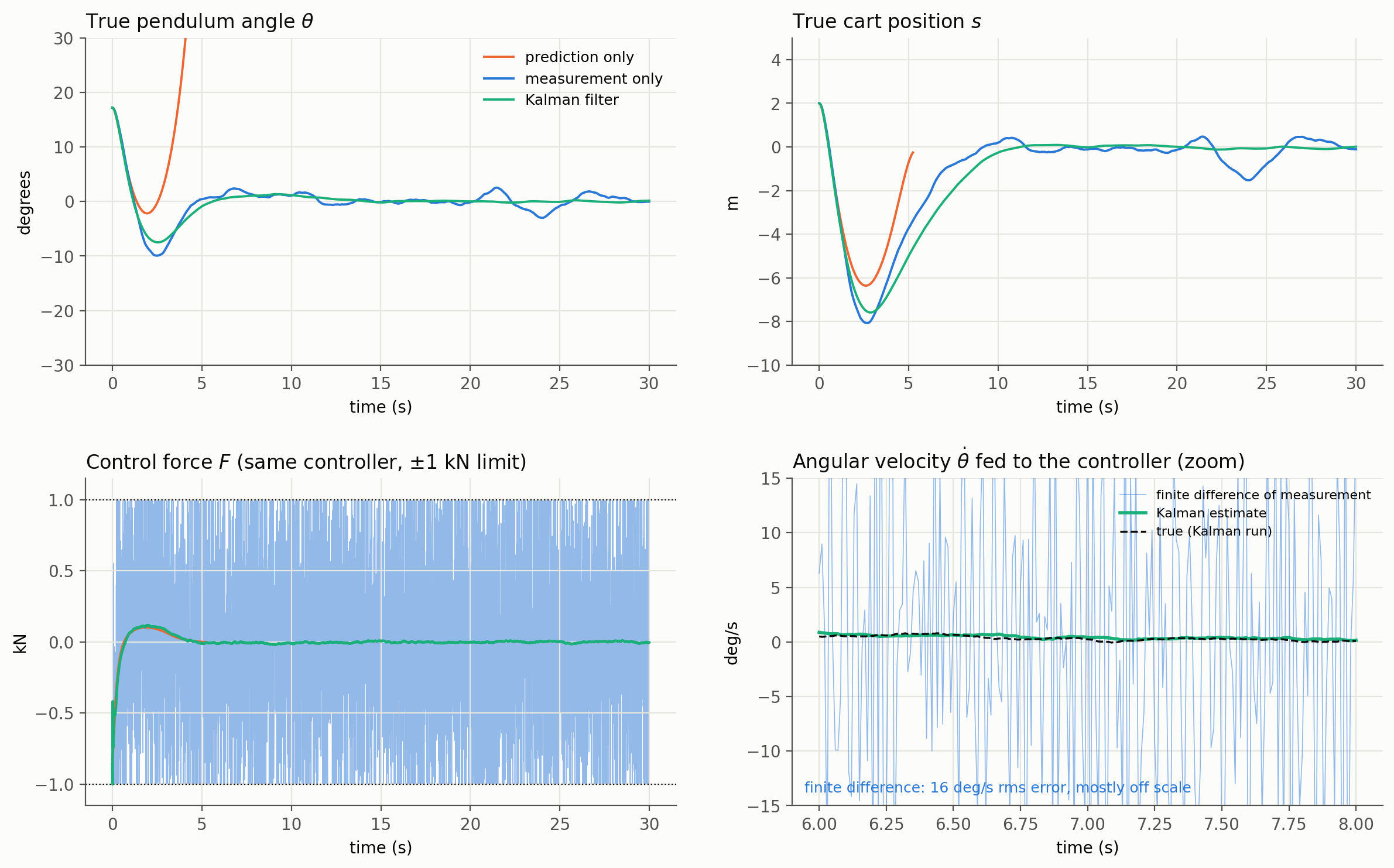
Prediction only starts from the right place, with a good model, and for the first second it looks just like the Kalman filter. But it never notices the gusts. Every unmeasured push makes the estimate drift away from reality, and because the pendulum is unstable, that error grows exponentially. The controller ends up balancing an imaginary pendulum while the real one falls over at 5.2 seconds.
Measurement only knows where the pendulum is, but not how fast it’s moving. Differentiating a noisy signal amplifies the noise: a 0.002 rad angle error divided by a 10 ms step becomes a velocity error of order $\sqrt{2} \times 0.002 / 0.01 \approx 0.28$ rad/s, or about 16°/s, exactly what we measured. The controller’s gain on $\dot{\theta}$ turns this into a force that chatters across the whole $\pm 1$ kN range, hitting the limit 28% of the time. The pendulum does stay up, but it keeps wobbling by a few degrees and the cart wanders around by more than a meter, because every time the motor is saturated, the controller is not the controller we designed.
NoteWith a noisier angle sensor of 0.01 rad (0.6°), the measurement-only case doesn’t survive at all: the force sits at the limit 87% of the time and the pendulum falls after about 10 seconds, while the Kalman filter still balances it. Saturation is what turns noisy estimates from “ugly” into “fatal”.
The Kalman filter gets the best of both: the angle estimate is 5 times more accurate than the raw sensor, and the velocity estimate, which we never measure, is accurate to 0.21°/s. The controller never hits the force limit, needs only 64 N rms (11 times less than measurement only), keeps the pendulum within 0.11° rms once settled (13 times better), and brings the cart from 2 m back to about 1 cm from home.