More Facts about IO Linearization
We are now aware of how to perform input-output linearization. To summarize:
- For an output with relative degree $r$, we are able to construct a feedback linearization mapping such that the input-output linearized system is of order $r$.
- The remaining states form a “zero plane” $Z$, and the zero dynamics on that plane determine the stability of the overall system.
Now, we can draw an obvious conclusion if the zero dynamics are indeed stable:
Theorem: If $z = 0$ is locally exponentially stable for the zero dynamics, $\dot{z} = q(0, z)$, then $u_{IO}, v$ locally exponentially stabilizes $x = 0$.
The proof is as follows:
Proof: The closed loop system is given by
$$ \begin{align*} \dot{\xi} &= A_{CL} \xi, A_{CL} = A - BK \\ \dot{z} &= q(\xi, z) \end{align*} $$where
$$ A_{CL} = \begin{pmatrix} 0 & 1 & 0 &\ldots & 0 \\ 0 & 0 & 1 & \ldots & 0 \\ \vdots & \vdots & \vdots & \ddots & \vdots \\ -k_1 & -k_2 & -k_3 & \ldots & -k_r \end{pmatrix} $$where $\Re{\lambda_i} < 0$ for all $i = 1, \ldots, r$. If we linearize the system at $\xi = z = 0$, we get the following:
$$ \frac{d}{dt} \begin{pmatrix} \delta \xi \\ \delta z \end{pmatrix} = \begin{pmatrix} A_{CL} & 0 \\ \frac{\partial q}{\partial \xi}(0, 0) & \frac{\partial q}{\partial z}(0, 0) \end{pmatrix} \begin{pmatrix} \delta \xi \\ \delta z \end{pmatrix} $$The matrix is Hurwitz, which completes the proof.
We notice that the relationship between the new states $\xi$ and original states $x$ is such that
$$ \xi = T(x)$$To verify if $T$ is a diffeomorphism, we introduce the following theorem:
Inverse Function Theorem: If a function $T: \mathbb{R}^n \to \mathbb{R}^n$, $T \in C^1$, has a Jacobian
$$ \frac{\partial T}{\partial x}(x_0) $$that is full rank, then $T^{-1}$ exists in a neighborhood of $T(x_0)$, and is continuous and differentiable.
Now let’s connect IO linearization back to feedback linearization. It’s not hard to see that if we can guarantee the zero dynamics to be stable, then the original system will be stable; the best way to make sure the zero dynamics are always stable is that the zero plane shrinks to just a point, and this is done if $r = n$. Therefore we have the following theorem:
Isidori, chapter 4: If a nonlinear system $\Sigma$ has a relative degree $r$ at $x_0$, then on the neighborhood of $x_0$, the functions
$$ \{ h(x), L_fh(x), \ldots, L_f^{r-1}h(x) \} $$are linearly independent. Then we can conclude that $\Sigma$ is feedback linearizable if and only if $\exists y = h(x)$ such that the output has relative degree $r = n$.
In short, if the output of the system has a relative degree equal to the system order, then the system is always linearizable. However, if the output has a relative degree smaller than the system degree, it’s possible that we didn’t pick a good output – how do we know if a system can in fact be feedback linearized? We’ll have to introduce some more new concepts to answer the question.
Introduction to Differential Geometry
Readers who have taken a class in general relativity may find these concepts familiar.
Manifold
Let $M$ be a non-empty subset of $\mathbb{R}^n$ and let $1 \le m < n$; then $M$ is an $m$-dimensional smooth Manifold of $\mathbb{R}^n$ if, $\forall p \in M$, $\exists r > 0$, $F:B_r(p) \to \mathbb{R}^{n-m}$ such that:
- \( M \cap B_r(p) = \{ x \in \mathbb{R}^n | F(x) = 0 \} \)
- $ F \in C^0 $
- $ \forall \bar{x} \in M \cap B_r(p)$, $\text{rank} \frac{\partial F}{\partial x}(\bar{x}) = n - m $
Intuitively, a manifold is a shape that “embeds” into a Euclidean space. We can always find a local mapping (also known as the “atlas”) to map the manifold into another local region in Euclidean space, given these two spaces have the same dimension.
Some well-known manifolds are:
- Circle, a 1D manifold in $\mathbb{R}^2$
- Möbius strip, a 2D manifold in $\mathbb{R}^3$
- Sphere, a 2D manifold in $\mathbb{R}^3$
- Klein bottle, a 2D manifold in $\mathbb{R}^4$
Tangent Space
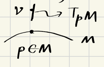
Let $M$ be a smooth manifold in $\mathbb{R}^n$ and let $p \in M$, suppose $F: B_r(p) \to \mathbb{R}^{n-m}$ satisfies the conditions in the definition of $M$. Then the Tangent Space of $M$ at $p$, denoted $T_pM$, is
$$ T_pM = \{ v \in \mathbb{R}^n | \frac{\partial F}{\partial x}(p) v = 0 \} = \mathcal{N}(\frac{\partial F}{\partial x}(p)) $$Note that $\text{dim}(T_pM) = m$.
Tangent Vector
The Tangent Vector is a vector in tangent space.
The relationship between a manifold, its tangent space and a tangent vector is illustrated below:
Vector Field
A Vector Field $f$ on a manifold $M$ assigns to each $p \in M$ a vector $f(p) \in T_pM$. Note that the vector field is $C^k$ if $f \in C^k$.
Lie Bracket
Given $f, g$ as two different vector fields, the Lie Bracket is defined as
$$ \begin{align*} [f, g](x) &= \frac{\partial g}{\partial x}(x) f(x) - \frac{\partial f}{\partial x}(x) g(x) \\ &= L_fg - L_gf \\ \end{align*} $$The Lie bracket can also be expressed in terms of the “adjoint” operator, i.e.:
$$ ad_f g(x) = [f, g](x) $$We can use the adjoint operator to express nested Lie brackets:
$$ \begin{align*} ad_f^2g(x) &= [f, ad_f g(x)] \\ &= [f, [f, g]](x) \end{align*} $$In general, we have
$$ ad_f^kg(x) = [f, ad_f^{k-1}g(x)] $$An example of Lie bracket calculation is as follows:
$$ \begin{align*} f &= \begin{pmatrix} x_2 \\ -\sin x_1 - x_2 \end{pmatrix} \\ g &= \begin{pmatrix} 0 \\ x_1 \end{pmatrix} \\ [f, g](x) &= L_fg - L_gf \\ &= \begin{pmatrix} 0 \\ x_2 \end{pmatrix} - \begin{pmatrix} x_1 \\ -x_1 \end{pmatrix} \\ &= \begin{pmatrix} -x_1 \\ x_2 + x_1 \end{pmatrix} \end{align*} $$Some useful properties of Lie bracket:
- $[f, f ] = 0$
- $[f, g] = -[g, f]$
- If $f$ and $g$ are constant vectors, then $[f, g] = 0$.
Now let’s consider a linear system $\dot{x} = Ax + Bu$. Expressed in control-affine form, we have
$$\begin{align*} \dot{x} &= f(x) + g(x)u \\ f(x) &= Ax \\ g(x) &= B \end{align*} $$$$ \begin{align*} ad_fg &= -AB \\ ad_f^2g &= A^2B \\ ad_f^3g &= -A^3B \\ \vdots \\ ad_f^kg &= (-1)^k A^k B \end{align*} $$Tangent Bundle
The Tangent Bundle of a manifold $M$ is defined as
$$ TM = \bigcup_{p \in M} T_pM $$That is, it’s the “bundle” of all tangent spaces at each point in the manifold.
Distribution
Suppose $f_1, f_2, \ldots, f_n$ are vector fields; the Distribution they span is defined as
$$ \Delta (x) = \text{span}\{f_1(x), f_2(x), \ldots, f_n(x)\} $$where at each point $x$, $\Delta(x)$ is a subspace of the tangent space $T_xM$.
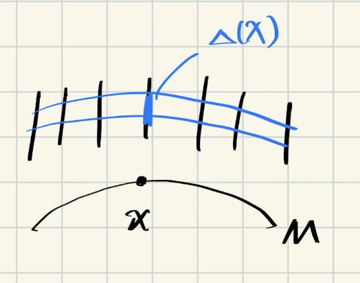
- $\Delta$ is a non-singular distribution if $\text{dim}(\Delta(x))$ is a constant $\forall x$.
- $\Delta$ is involutive if $$ \forall f, g \in \Delta \Rightarrow [f, g] \in \Delta $$
Let’s consider the following example:
$$ \begin{align*} f_1 &= \begin{pmatrix} 2x_2 \\ 1 \\ 0 \end{pmatrix} \\ f_2 &= \begin{pmatrix} 1 \\ 0 \\ x_2 \end{pmatrix} \\ \Delta &= \text{span}\{f_1, f_2\} \end{align*} $$Because $\text{dim}\Delta(x) = 2$ for all $x$, the distribution $\Delta$ is non-singular.
$\Delta$ is involutive if and only if
$$ [f_1, f_2] = \begin{pmatrix} 0 \\ 0 \\ 1 \end{pmatrix} \in \Delta $$i.e. $\text{rank}(f_1, f_2, [f_1, f_2]) = 2 \quad \forall x$. Unfortunately the rank is 3, therefore $\Delta$ is not involutive.
Feedback Linearizability
With all these mathematical definitions, we are finally able to determine whether a nonlinear system can actually be feedback linearized, using the following theorem:
A nonlinear system $\Sigma$ is feedback linearizable if and only if:
- $[g(x), ad_fg(x), \ldots, ad_f^{n-1}g(x) ]$ has rank $n$, $\forall x$. This condition guarantees controllability.
- \( \Delta = \text{span}\{g, ad_fg, \ldots, ad_f^{n-2}g\} \) is involutive.
Once we have determined that the system is feedback linearizable, the next step is to look for the specific output with relative degree $n$. From our earlier discussion, we are looking for a function $y = h(x)$ such that it meets the following conditions:
$$\begin{align*} \begin{cases} L_gh = L_gL_fh = \ldots = L_gL_f^{n-2}h = 0 \quad \forall x \\ L_gL_f^{n-1}h \neq 0 \end{cases} \end{align*} $$In fact, these two conditions are equivalent to the following two conditions:
$$\begin{align*} \begin{cases} L_gh = L_{ad_fg}h = \ldots = L_{ad_f^{n-2}g}h = 0 \quad \forall x \\ L_{ad_f^{n-1}g}h \neq 0 \end{cases} \end{align*} $$The advantage of the latter formulation is that we can write the first condition as:
$$ \frac{\partial h}{\partial x} \begin{pmatrix} g(x) & ad_fg(x) & \cdots & ad_f^{n-2}g(x) \end{pmatrix} = 0 $$The important fact here is that the solution to this partial differential equation exists only if \( \Delta = \text{span}\{g, ad_fg, \ldots, ad_f^{n-2}g\} \) is involutive, according to the Frobenius theorem.
To prove that the two conditions are indeed equivalent, we use the following lemma:
Lemma: If $L_gh = L_gL_f h = \ldots = L_gL_f^{n-2}h = 0$ for all $x \in B_\delta (x_0)$, then
$$L_gL_f^kh = (-1)^k L_{ad_f^kg}h, \quad \forall k = 0,1,\ldots, n-1$$
This lemma can be proven using induction, and we skip the full proof here.
In this chapter, we discussed the conditions for a nonlinear system to be fully feedback linearizable. In the final chapter, we’ll give some examples and extend to multi-input multi-output case.